clusterprolifer go kegg msigdbr 富集分析应该使用哪个数据集，GO?KEGG?Hallmark？

本文主要是介绍clusterprolifer go kegg msigdbr 富集分析应该使用哪个数据集，GO?KEGG?Hallmark？，希望对大家解决编程问题提供一定的参考价值，需要的开发者们随着小编来一起学习吧！

关注微信：生信小博士

5 Overview of enrichment analysis

Chapter 5 Overview of enrichment analysis | Biomedical Knowledge Mining using GOSemSim and clusterProfiler

5.1.2 Gene Ontology (GO)

Gene Ontology defines concepts/classes used to describe gene function, and relationships between these concepts. It classifies functions along three aspects:

MF: Molecular Function
- molecular activities of gene products
CC: Cellular Component
- where gene products are active
BP: Biological Process
- pathways and larger processes made up of the activities of multiple gene products

GO terms are organized in a directed acyclic graph, where edges between terms represent parent-child relationship.

5.1.3 Kyoto Encyclopedia of Genes and Genomes (KEGG)

KEGG is a collection of manually drawn pathway maps representing molecular interaction and reaction networks. These pathways cover a wide range of biochemical processes that can be divided into 7 broad categories:

Metabolism
Genetic information processing
Environmental information processing
Cellular processes
Organismal systems
Human diseases
Drug development.

5.1.4 Other gene sets

GO and KEGG are the most frequently used for functional analysis. They are typically the first choice because of their long-standing curation and availability for a wide range of species.

Other gene sets include but are not limited to Disease Ontology (DO), Disease Gene Network (DisGeNET), wikiPathways, Molecular Signatures Database (MSigDb).

富集分析的原理

Over Representation Analysis (ORA)和Gene Set Enrichment Analysis (GSEA)是用于分析基因表达数据的两种常见方法。ORA基于预定义的基因集，用超几何分布计算差异表达基因与该基因集中的基因数之间的显著性，适用于已知基因集和差异表达较大情况。GSEA考虑所有基因，根据基因在表型排序上的变化来寻找整个基因集是否显著富集，比ORA更适用于寻找微小但协调变化的基因集。GSEA还包括较新的leading edge analysis和core enriched genes等功能，能够帮助确定影响基因富集的关键基因。两种方法各有优缺点，在不同的研究问题中可以灵活选用。

5.2 原理1 Over Representation Analysis

Example: Suppose we have 17,980 genes detected in a Microarray study and 57 genes were differentially expressed. Among the differentially expressed genes, 28 are annotated to a gene set1.

d <- data.frame(gene.not.interest=c(2613, 15310), gene.in.interest=c(28, 29))
row.names(d) <- c("In_category", "not_in_category")
d

##                 gene.not.interest gene.in.interest
## In_category                  2613               28
## not_in_category             15310               29

Whether the overlap(s) of 25 genes are significantly over represented in the gene set can be assessed using a hypergeometric distribution. This corresponds to a one-sided version of Fisher’s exact test.

fisher.test(d, alternative = "greater")

5.3 原理2 Gene Set Enrichment Analysis

ORA的方法，对于差异明显的对比结果较好，但是对于差异小的结果不好

A common approach to analyzing gene expression profiles is identifying differentially expressed genes that are deemed interesting. The ORA enrichment analysis is based on these differentially expressed genes. This approach will find genes where the difference is large and will fail where the difference is small, but evidenced in coordinated way in a set of related genes. Gene Set Enrichment Analysis (GSEA)(Subramanian et al. 2005) directly addresses this limitation. All genes can be used in GSEA; GSEA aggregates the per gene statistics across genes within a gene set, therefore making it possible to detect situations where all genes in a predefined set change in a small but coordinated way. This is important since it is likely that many relevant phenotypic differences are manifested by small but consistent changes in a set of genes.

Genes are ranked based on their phenotypes. Given apriori defined set of gene S (e.g., genes sharing the same DO category), the goal of GSEA is to determine whether the members of S are randomly distributed throughout the ranked gene list (L) or primarily found at the top or bottom.

There are three key elements of the GSEA method:

Calculation of an Enrichment Score.
- The enrichment score (ES) represents the degree to which a set S is over-represented at the top or bottom of the ranked list L. The score is calculated by walking down the list L, increasing a running-sum statistic when we encounter a gene in S and decreasing when it is not encountered. The magnitude of the increment depends on the gene statistics (e.g., correlation of the gene with phenotype). The ES is the maximum deviation from zero encountered in the random walk; it corresponds to a weighted Kolmogorov-Smirnov(KS)-like statistic (Subramanian et al. 2005).
Esimation of Significance Level of ES.
- The p-value of the ES is calculated using a permutation test. Specifically, we permute the gene labels of the gene list L and recompute the ES of the gene set for the permutated data, which generate a null distribution for the ES. The p-value of the observed ES is then calculated relative to this null distribution.
Adjustment for Multiple Hypothesis Testing.
- When the entire gene sets are evaluated, the estimated significance level is adjusted to account for multiple hypothesis testing and also q-values are calculated for FDR control.

We implemented the GSEA algorithm proposed by Subramanian (Subramanian et al. 2005). Alexey Sergushichev implemented an algorithm for fast GSEA calculation in the fgsea (Korotkevich, Sukhov, and Sergushichev 2019) package. In our packages (clusterProfiler, DOSE, meshes and ReactomePA), users can use the GSEA algorithm implemented in DOSE or fgsea by specifying the parameter by="DOSE" or by="fgsea". By default, the fgsea method will be used since it is much more faster.

5.4 原理3 Leading edge analysis and core enriched genes

Leading edge analysis reports Tags to indicate the percentage of genes contributing to the enrichment score, List to indicate where in the list the enrichment score is attained and Signal for enrichment signal strength.

It would also be very interesting to get the core enriched genes that contribute to the enrichment. Our packages (clusterProfiler, DOSE, meshes and ReactomePA) support leading edge analysis and report core enriched genes in GSEA analysis.

详细的富集分析使用范围及其原理

1 GO 富集

GO comprises three orthogonal ontologies, i.e. molecular function (MF), biological process (BP), and cellular component (CC).

6.1 Supported organisms

GO analyses (groupGO(), enrichGO() and gseGO()) support organisms that have an OrgDb object available (see also session 2.2).

If a user has GO annotation data (in a data.frame format with the first column as gene ID and the second column as GO ID), they can use the enricher() and GSEA() functions to perform an over-representation test and gene set enrichment analysis.

If the genes are annotated by direction annotation, they should also be annotated by their ancestor GO nodes (indirect annotation). If a user only has direct annotation, they can pass their annotation to the buildGOmap function, which will infer indirect annotation and generate a data.frame that is suitable for both enricher() and GSEA().

6.2 groupGo是对基因的分类

In clusterProfiler, the groupGO() function is designed for gene classification based on GO distribution at a specific level. Here we use the dataset geneList provided by DOSE.

library(clusterProfiler)
data(geneList, package="DOSE")
gene <- names(geneList)[abs(geneList) > 2]# Entrez gene ID
head(gene)

## [1] "4312"  "8318"  "10874" "55143" "55388" "991"

ggo <- groupGO(gene     = gene,OrgDb    = org.Hs.eg.db,ont      = "CC",level    = 3,readable = TRUE)head(ggo)

6.3 enrichGO()是通过ORA对基因进行富集分析

The clusterProfiler package implements enrichGO() for gene ontology over-representation test.

ego <- enrichGO(gene          = gene,universe      = names(geneList),OrgDb         = org.Hs.eg.db,ont           = "CC",pAdjustMethod = "BH",pvalueCutoff  = 0.01,qvalueCutoff  = 0.05,readable      = TRUE)
head(ego)

gene.df <- bitr(gene, fromType = "ENTREZID",toType = c("ENSEMBL", "SYMBOL"),OrgDb = org.Hs.eg.db)ego2 <- enrichGO(gene         = gene.df$ENSEMBL,OrgDb         = org.Hs.eg.db,keyType       = 'ENSEMBL',ont           = "CC",pAdjustMethod = "BH",pvalueCutoff  = 0.01,qvalueCutoff  = 0.05)
head(ego2, 3)

6.4 `gseGO()` 是对基因集进行gsea分析，而GSEA是对基因列表基因gsea分析？？

The clusterProfiler package provides the gseGO() function for gene set enrichment analysis using gene ontology.

ego3 <- gseGO(geneList     = geneList,OrgDb        = org.Hs.eg.db,ont          = "CC",minGSSize    = 100,maxGSSize    = 500,pvalueCutoff = 0.05,verbose      = FALSE)

The format of input data, geneList, was documented in the FAQ. Beware that only gene Set size in [minGSSize, maxGSSize] will be tested.

A.1 How to prepare your own geneList

GSEA analysis requires a ranked gene list, which contains three features:

numeric vector: fold change or other type of numerical variable
named vector: every number has a name, the corresponding gene ID
sorted vector: number should be sorted in decreasing order

If you import your data from a csv file, the file should contains two columns, one for gene ID (no duplicated ID allowed) and another one for fold change. You can prepare your own geneList via the following command:

d = read.csv(your_csv_file)
## assume 1st column is ID
## 2nd column is FC## feature 1: numeric vector
geneList = d[,2]## feature 2: named vector
names(geneList) = as.character(d[,1])## feature 3: decreasing orde
geneList = sort(geneList, decreasing = TRUE)

7.2 KEGG pathway ORA

Input ID type can be kegg, ncbi-geneid, ncbi-proteinid or uniprot (see also session 16.1.2). Unlike enrichGO(), there is no readable parameter for enrichKEGG(). However, users can use the setReadable() function if there is an OrgDb available for the species.

data(geneList, package="DOSE")
gene <- names(geneList)[abs(geneList) > 2]kk <- enrichKEGG(gene         = gene,organism     = 'hsa',pvalueCutoff = 0.05)
head(kk)

##                ID                                                   Description
## hsa04110 hsa04110                                                    Cell cycle
## hsa04114 hsa04114                                                Oocyte meiosis
## hsa04218 hsa04218                                           Cellular senescence
## hsa04061 hsa04061 Viral protein interaction with cytokine and cytokine receptor
## hsa03320 hsa03320                                        PPAR signaling pathway
## hsa04914 hsa04914                       Progesterone-mediated oocyte maturation
##          GeneRatio  BgRatio       pvalue     p.adjust       qvalue
## hsa04110     11/94 126/8142 1.829412e-07 3.841764e-05 3.774365e-05
## hsa04114     10/94 131/8142 2.368439e-06 2.486861e-04 2.443231e-04
## hsa04218     10/94 156/8142 1.135672e-05 7.949704e-04 7.810235e-04
## hsa04061      8/94 100/8142 1.821466e-05 9.562698e-04 9.394931e-04
## hsa03320      7/94  75/8142 2.285993e-05 9.601169e-04 9.432728e-04
## hsa04914      7/94 102/8142 1.651911e-04 5.781690e-03 5.680256e-03
##                                                      geneID Count
## hsa04110 8318/991/9133/890/983/4085/7272/1111/891/4174/9232    11
## hsa04114    991/9133/983/4085/51806/6790/891/9232/3708/5241    10
## hsa04218     2305/4605/9133/890/983/51806/1111/891/776/3708    10
## hsa04061           3627/10563/6373/4283/6362/6355/9547/1524     8
## hsa03320                 4312/9415/9370/5105/2167/3158/5346     7
## hsa04914                    9133/890/983/4085/6790/891/5241     7

7.3 KEGG pathway GSEA

kk2 <- gseKEGG(geneList     = geneList,organism     = 'hsa',minGSSize    = 120,pvalueCutoff = 0.05,verbose      = FALSE)
head(kk2)

##                ID                              Description setSize
## hsa05169 hsa05169             Epstein-Barr virus infection     193
## hsa04613 hsa04613  Neutrophil extracellular trap formation     130
## hsa05166 hsa05166  Human T-cell leukemia virus 1 infection     202
## hsa04510 hsa04510                           Focal adhesion     190
## hsa04218 hsa04218                      Cellular senescence     141
## hsa05170 hsa05170 Human immunodeficiency virus 1 infection     189
##          enrichmentScore       NES       pvalue     p.adjust      qvalues rank
## hsa05169       0.4335010  1.962039 5.505487e-08 4.239225e-06 2.839672e-06 2820
## hsa04613       0.4496569  1.934454 6.345081e-06 2.442856e-04 1.636363e-04 2575
## hsa05166       0.3893613  1.755469 1.357530e-05 3.484327e-04 2.333999e-04 1955
## hsa04510      -0.4169068 -1.691234 2.771385e-05 5.334917e-04 3.573629e-04 2183
## hsa04218       0.4115945  1.783044 5.168200e-05 7.959028e-04 5.331406e-04 1155
## hsa05170       0.3711150  1.677643 1.118012e-04 1.229814e-03 8.237986e-04 3178
##                            leading_edge
## hsa05169 tags=39%, list=23%, signal=31%
## hsa04613 tags=37%, list=21%, signal=30%
## hsa05166 tags=26%, list=16%, signal=22%
## hsa04510 tags=27%, list=17%, signal=22%
## hsa04218  tags=17%, list=9%, signal=16%
## hsa05170 tags=38%, list=25%, signal=29%
##                                                                                                                                                                                                                                                                                                                                                                                core_enrichment
## hsa05169 3627/890/6890/9636/898/9134/6502/6772/3126/3112/4609/917/5709/1869/3654/919/915/4067/4938/864/4940/5713/5336/11047/3066/54205/1871/578/1019/637/916/3383/4939/10213/23586/4793/5603/7979/7128/6891/930/5714/3452/6850/5702/4794/7124/3569/7097/5708/2208/8772/3119/5704/7186/5971/3135/1380/958/5610/4792/10018/8819/3134/10379/9641/1147/5718/6300/3109/811/5606/2923/3108/5707/1432
## hsa04613                                                                                                                                      820/366/51311/64581/3015/85236/55506/8970/8357/1535/2359/5336/4688/92815/3066/8336/292/1991/3689/8345/5603/4689/5880/10105/1184/6404/3018/6850/5604/3014/7097/1378/8290/1536/834/5605/1183/728/2215/8335/5594/9734/3674/5578/5582/7417/8331/6300
## hsa05166                                                                                                                      991/9133/890/4085/7850/1111/9232/8061/701/9700/898/4316/9134/3932/3559/3126/3112/4609/3561/917/1869/1029/915/114/2005/5902/55697/1871/1031/2224/292/1019/3689/916/3383/11200/706/3600/6513/3601/468/5604/7124/1030/3569/4049/4055/10393/3119/5901/5971/1959/3135
## hsa04510                                                                                                                   5595/5228/7424/1499/4636/83660/7059/5295/1288/23396/3910/3371/3082/1291/394/3791/7450/596/3685/1280/3675/595/2318/3912/1793/1278/1277/1293/10398/55742/2317/7058/25759/56034/3693/3480/5159/857/1292/3908/3909/63923/3913/1287/3679/7060/3479/10451/80310/1311/1101
## hsa04218                                                                                                                                                                                                                                                                 2305/4605/9133/890/983/51806/1111/891/993/3576/1978/898/9134/4609/1869/1029/22808/1871/5499/91860/292/1019/11200/1875
## hsa05170                   9133/9582/983/51806/1111/891/6890/200315/917/3654/919/915/5336/54205/91860/578/995/25939/637/1234/916/5603/2792/5880/6891/6921/3452/5604/7124/9978/7097/7852/8772/1174/7186/3135/164/60489/2787/356/7133/5605/27350/6199/1642/5594/4792/3134/5578/4893/8454/5582/2786/1147/3984/6300/200316/811/5606/2923/4775/162/1432/2784/836/5747/5058/3106/2770/5534/5579/4615

7.4 KEGG module ORA. 这里的module指的是msigdb种收集的其他kegg内容，共有

KEGG Module is a collection of manually defined function units. In some situation, KEGG Modules have a more straightforward interpretation.

mkk <- enrichMKEGG(gene = gene,organism = 'hsa',pvalueCutoff = 1,qvalueCutoff = 1)
head(mkk)

3.KEGG 分类备注

KEGG Pathway可以进行分类汇总。

在KEGG官网（KEGG PATHWAY Database）中，将通路分成了7类：

1. Metabolism （代谢）

2. Genetic Information Processing （遗传信息处理）

3. Environmental Information Processing （环境信息处理）

4. Cellular Processes （细胞过程）

5. Organismal Systems （生物系统）

6. Human Diseases （人类疾病）

7. Drug Development （药物开发）

做出一个分类汇总图，这样可以在更上一层级研究pathway。主要应用于特殊物种的denovo测序注释，也可以应用于我们常规的pathway富集分析。

7.5 KEGG module gene set enrichment analysis

mkk2 <- gseMKEGG(geneList = geneList,organism = 'hsa',pvalueCutoff = 1)
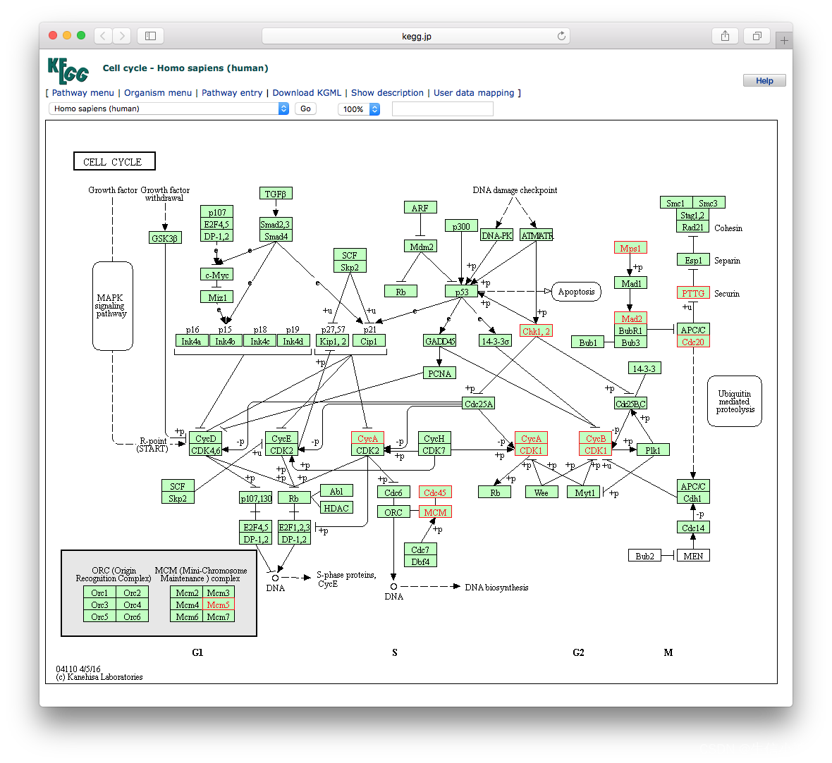
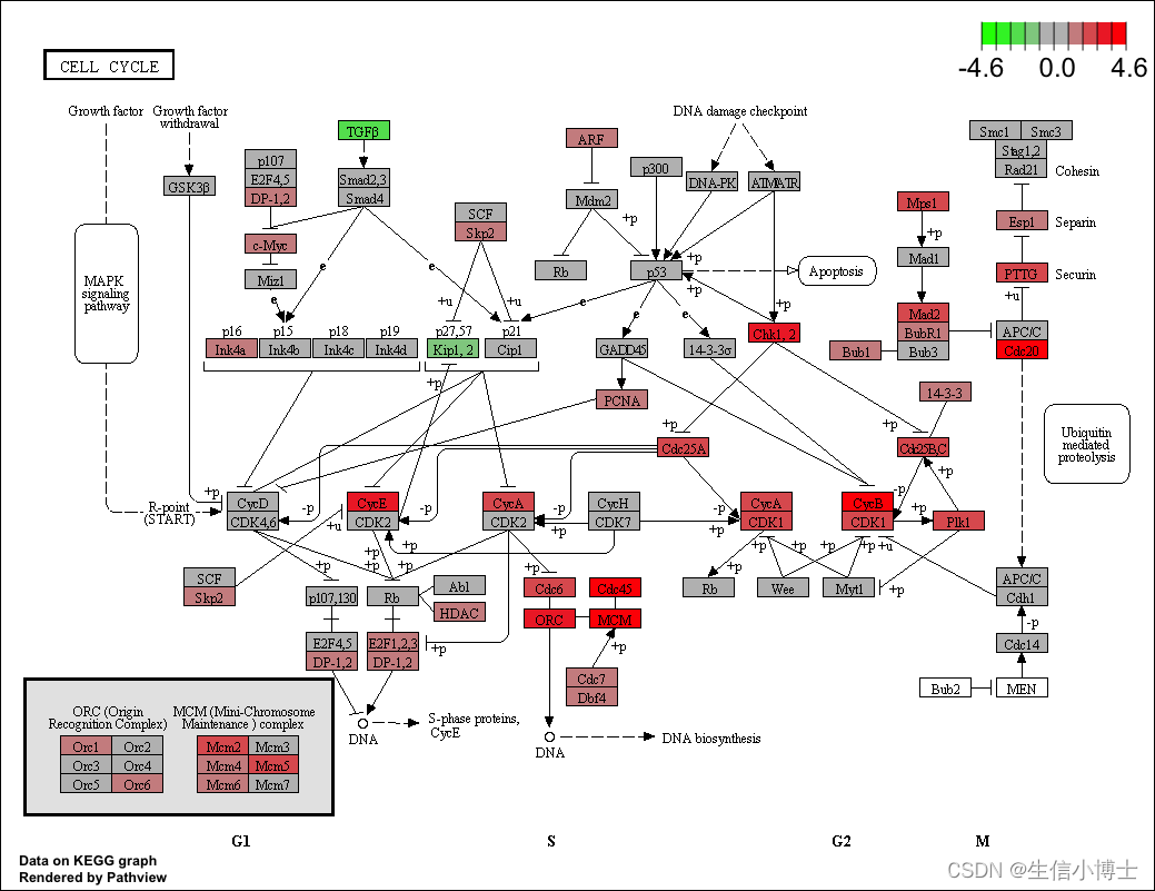
head(mkk2)

通路可视化

library("pathview") hsa04110 <- pathview(gene.data = geneList, pathway.id = "hsa04110", species = "hsa", limit = list(gene=max(abs(geneList)), cpd=1))

browseKEGG(kk, 'hsa04110')