数据分析实战(八)：北上广深租房图鉴

项目主要爬取北上广深链家网全部租房房源数据，并且得出租金分布、租房考虑因素等建议。

首先奉上爬虫demo，如果有直接需要数据的请评论留言，会分享。

import os
import re
import time
import requests
from pymongo import MongoClient
from info import rent_type, city_infoclass Rent(object):"""初始化函数，获取租房类型（整租、合租）、要爬取的城市分区信息以及连接mongodb数据库"""def __init__(self):self.rent_type = rent_typeself.city_info = city_infohost = os.environ.get('MONGODB_HOST', '127.0.0.1')  # 本地数据库port = os.environ.get('MONGODB_PORT', '27017')  # 数据库端口mongo_url = 'mongodb://{}:{}'.format(host, port)mongo_db = os.environ.get('MONGODB_DATABASE', 'Lianjia')client = MongoClient(mongo_url)self.db = client[mongo_db]self.db['zufang'].create_index('m_url', unique=True)  # 以m端链接为主键进行去重def get_data(self):"""爬取不同租房类型、不同城市各区域的租房信息:return: None"""for ty, type_code in self.rent_type.items():  # 整租、合租for city, info in self.city_info.items():  # 城市、城市各区的信息for dist, dist_py in info[2].items():  # 各区及其拼音res_bc = requests.get('https://m.lianjia.com/chuzu/{}/zufang/{}/'.format(info[1], dist_py))pa_bc = r"data-type=\"bizcircle\" data-key=\"(.*)\" class=\"oneline \">"bc_list = re.findall(pa_bc, res_bc.text)self._write_bc(bc_list)bc_list = self._read_bc()  # 先爬取各区的商圈，最终以各区商圈来爬数据，如果按区爬，每区最多只能获得2000条数据if len(bc_list) > 0:for bc_name in bc_list:idx = 0has_more = 1while has_more:try:url = 'https://app.api.lianjia.com/Rentplat/v1/house/list?city_id={}&condition={}' \'/rt{}&limit=30&offset={}&request_ts={}&scene=list'.format(info[0],bc_name,type_code,idx*30,int(time.time()))res = requests.get(url=url, timeout=10)print('成功爬取{}市{}-{}的{}第{}页数据！'.format(city, dist, bc_name, ty, idx+1))item = {'city': city, 'type': ty, 'dist': dist}self._parse_record(res.json()['data']['list'], item)total = res.json()['data']['total']idx += 1if total/30 <= idx:has_more = 0# time.sleep(random.random())except:print('链接访问不成功，正在重试！')def _parse_record(self, data, item):"""解析函数，用于解析爬回来的response的json数据:param data: 一个包含房源数据的列表:param item: 传递字典:return: None"""if len(data) > 0:for rec in data:item['bedroom_num'] = rec.get('frame_bedroom_num')item['hall_num'] = rec.get('frame_hall_num')item['bathroom_num'] = rec.get('frame_bathroom_num')item['rent_area'] = rec.get('rent_area')item['house_title'] = rec.get('house_title')item['resblock_name'] = rec.get('resblock_name')item['bizcircle_name'] = rec.get('bizcircle_name')item['layout'] = rec.get('layout')item['rent_price_listing'] = rec.get('rent_price_listing')item['house_tag'] = self._parse_house_tags(rec.get('house_tags'))item['frame_orientation'] = rec.get('frame_orientation')item['m_url'] = rec.get('m_url')item['rent_price_unit'] = rec.get('rent_price_unit')try:res2 = requests.get(item['m_url'], timeout=5)pa_lon = r"longitude: '(.*)',"pa_lat = r"latitude: '(.*)'"pa_distance = r"<span class=\"fr\">(\d*)米</span>"item['longitude'] = re.findall(pa_lon, res2.text)[0]item['latitude'] = re.findall(pa_lat, res2.text)[0]distance = re.findall(pa_distance, res2.text)if len(distance) > 0:item['distance'] = distance[0]else:item['distance'] = Noneexcept:item['longitude'] = Noneitem['latitude'] = Noneitem['distance'] = Noneself.db['zufang'].update_one({'m_url': item['m_url']}, {'$set': item}, upsert=True)print('成功保存数据:{}!'.format(item))@staticmethoddef _parse_house_tags(house_tag):"""处理house_tags字段，相当于数据清洗:param house_tag: house_tags字段的数据:return: 处理后的house_tags"""if len(house_tag) > 0:st = ''for tag in house_tag:st += tag.get('name') + ' 'return st.strip()@staticmethoddef _write_bc(bc_list):"""把爬取的商圈写入txt，为了整个爬取过程更加可控:param bc_list: 商圈list:return: None"""with open('bc_list.txt', 'w') as f:for bc in bc_list:f.write(bc+'\n')@staticmethoddef _read_bc():"""读入商圈:return: None"""with open('bc_list.txt', 'r') as f:return [bc.strip() for bc in f.readlines()]if __name__ == '__main__':rent = Rent()rent.get_data()

其中的info.py文件

rent_type = {'整租': 200600000001, '合租': 200600000002}city_info = {'北京': [110000, 'bj', {'东城': 'dongcheng', '西城': 'xicheng', '朝阳': 'chaoyang', '海淀': 'haidian','丰台': 'fengtai', '石景山': 'shijingshan', '通州': 'tongzhou', '昌平': 'changping','大兴': 'daxing', '亦庄开发区': 'yizhuangkaifaqu', '顺义': 'shunyi', '房山': 'fangshan','门头沟': 'mentougou', '平谷': 'pinggu', '怀柔': 'huairou', '密云': 'miyun','延庆': 'yanqing'}],'上海': [310000, 'sh', {'静安': 'jingan', '徐汇': 'xuhui', '黄浦': 'huangpu', '长宁': 'changning','普陀': 'putuo', '浦东': 'pudong', '宝山': 'baoshan', '闸北': 'zhabei','虹口': 'hongkou','杨浦': 'yangpu', '闵行': 'minhang', '金山': 'jinshan','嘉定': 'jiading','崇明': 'chongming', '奉贤': 'fengxian', '松江': 'songjiang','青浦': 'qingpu'}],'广州': [440100, 'gz', {'天河': 'tianhe', '越秀': 'yuexiu', '荔湾': 'liwan', '海珠': 'haizhu', '番禺': 'panyu','白云': 'baiyun', '黄埔': 'huangpu', '从化': 'conghua', '增城': 'zengcheng','花都': 'huadu', '南沙': 'nansha'}],'深圳': [440300, 'sz', {'罗湖区': 'luohuqu', '福田区': 'futianqu', '南山区': 'nanshanqu','盐田区': 'yantianqu', '宝安区': 'baoanqu', '龙岗区': 'longgangqu','龙华区': 'longhuaqu', '光明区': 'guangmingqu', '坪山区': 'pingshanqu','大鹏新区': 'dapengxinqu'}]}

正式开始分析之旅

数据介绍

_id 唯一ID
bathroom_num
bedroom_num 卧室数量
bizcircle_name
city 城市
dist 区
distance 距离地铁距离
frame_orientation
hall_num 大厅数量
house_tag 房屋标签
house_title 房屋名称
latitude 维度
layout 布局类型
longitude 经度
m_url 网站来源
rent_area 出租面积
rent_price_listing 价格
rent_price_unit 出租价格单位
resblock_name 小区名称
type 出租类型

数据预处理

import pandas as pd
import numpy as np
import matplotlib.pyplot as plt
import seaborn as sns
from pylab import mpl# 预设值
mpl.rcParams['font.sans-serif'] = ['SimHei']  # 解决seaborn中文字体显示问题
plt.style.use('ggplot')
plt.rc('figure', figsize=(10, 10))  # 把plt默认的图片size调大一点
plt.rcParams["figure.dpi"] = mpl.rcParams['axes.unicode_minus'] = False  # 解决保存图像是负号'-'显示为方块的问题data = pd.read_csv('data_sample.csv')
print(data.info())'''
# 会采样数据，本数据已经采样完成，故不再重复此操作
# 每个城市各采样3000条数据，保存为csv文件
data_sample = pd.concat([data[data['city'] == city].sample(3000) for city in ['北京', '上海', '广州', '深圳']])
data_sample.to_csv('data_sample.csv', index=False)
'''

清洗数据

# 数据清洗(按列清理)
# 1. 去掉“_id”列
data = data.drop(columns='_id')# 2. 查看bathroom_num
print('通过浴室检验异常值：')
print(data['bathroom_num'].unique())
# 这里我们会看到，卫生间多的 都是合租房,没有异常值
# print(data[data['bathroom_num'].isin(['8', '9', '11'])])
print('\n')# 3. bedroom_num
print('通过卧室检验异常值：')
print(data['bedroom_num'].unique())
# 没有异常数据，只是很多10室以上都是专门用来合租的
# print(data[data['bedroom_num'].isin(['10', '11', '12', '13', '14', '15', '20'])])
print('\n')# 4. distance
data['frame_orientation'].unique()  # 这个数据太乱了，要用的时候再处理叭# 5. hall_num
print('通过大厅检验异常值：')
print(data['hall_num'].unique())  # 无异常值
print('\n')# 6. rent_area
# print(data.sample(5)['rent_area'])  # 随机查看# rent_area字段有些填写的是一个范围，比如23-25平房米，后期转换成“float”类型的时候不好转换，考虑取平均值
def get_aver(data):if isinstance(data, str) and '-' in data:low, high = data.split('-')return (int(low)+int(high))/2else:return int(data)data['rent_area'] = data['rent_area'].apply(get_aver)print('通过面积检验异常值：')
print(data[data['rent_area'] < 5])    # 输出,无异常值
print('\n')# 7. rent_price_unit
print(data['rent_price_unit'].unique())# 租金都是以“元/月”计算的，所以这一列没用了，可以删了
data = data.drop(columns='rent_price_unit')# 查看是否删除成功
# print(data.info())
print('\n')# 8. rent_price_listing
# print(data[data['rent_price_listing'].str.contains('-')].sample(3))# 我们可以看到：价格是有区间的，需要按照处理rent_area一样的方法处理
data['rent_price_listing'] = data['rent_price_listing'].apply(get_aver)# 重点：数据类型转换
for col in ['bathroom_num', 'bedroom_num', 'hall_num', 'rent_price_listing']:data[col] = data[col].astype(int)# 'distance', 'latitude', 'longitude'因为有None，需另外处理
def to_int(data):if data.isnull():  # nan是float类型，在python3.中无法强制转化为intreturn np.nanelse:return int(data)def to_float(data):if data is None or data == '':return np.nanelse:return float(data)# 这里都转化为float
data['distance'] = data['distance'].apply(to_float)
data['latitude'] = data['latitude'].apply(to_float)
data['longitude'] = data['longitude'].apply(to_float)print('\n')
print('数据清洗结束，查看数据：')
print(data.info())

问题：
各城市的租房分布怎么样？
城市各区域的房价分布怎么样？
距离地铁口远近有什么关系？
房屋大小对价格的影响如何？
租个人房源好还是公寓好？
精装和简装对房子价格的影响
北方集中供暖对价格的影响
北上广深租房时都看重什么？

1.各城市的租房分布怎么样？

def get_city_zf_loc(city, city_short, col=['longitude', 'latitude', 'dist'], data=data):file_name = 'data_' + city_short + '_latlon.csv'data_latlon = data.loc[data['city'] == city, col].dropna(subset=['latitude', 'longitude'])data_latlon['longitude'] = data_latlon['longitude'].astype(str)data_latlon['latitude'] = data_latlon['latitude'].astype(str)data_latlon['latlon'] = data_latlon['longitude'].str.cat(data_latlon['latitude'], sep=',')# data_latlon.to_csv(file_name, index=False) # 分别保存各城市，以后精细分析print(city+'的数据一共有{}条'.format(data_latlon.shape[0]))# 分别是：经度 纬度 区
get_city_zf_loc('北京', 'bj', ['longitude', 'latitude', 'dist'])
get_city_zf_loc('上海', 'sh', ['longitude', 'latitude', 'dist'])
get_city_zf_loc('广州', 'gz', ['longitude', 'latitude', 'dist'])
get_city_zf_loc('深圳', 'sz', ['longitude', 'latitude', 'dist'])# 画出北京各区分布
fig = plt.figure(dpi=300)
data.dropna(subset=['latitude', 'longitude'])[data['city'] == '北京']['dist'].value_counts(ascending=True).plot.barh()
plt.show()fig = plt.figure(dpi=300)
data.dropna(subset=['latitude', 'longitude'])[data['city'] =='上海']['dist'].value_counts(ascending=True).plot.barh()
plt.show()# 其余两个城市的图在这里不画啦~~

2.城市各区域的房价分布怎么样？

#  我们先看一下两个城市的单价分布情况
data['aver_price'] = data['rent_price_listing'] / data['rent_area']  # 平方单价
sns.distplot((data[data['city'] == '北京']['aver_price']), bins=100, label='Bei Jing')
plt.legend()
plt.show()data['aver_price'] = data['rent_price_listing'] / data['rent_area']
sns.distplot((data[data['city'] == '上海']['aver_price']), bins=100, label='Shang Hai')
plt.legend()
plt.show()

# 由于平均租金基本上都集中在250元/平米/月以内，所以选取这部分数据绘制热力图
# 这个函数可以得到的我们需要的数据（按城市分开）
def get_city_zf_aver_price(city, city_short, col=['longitude', 'latitude', 'aver_price'], data=data):file_name = 'data_' + city_short + '_aver_price.csv'data_latlon = data.loc[(data['city'] == city) & (data['aver_price'] <= 250), col].dropna(subset=['latitude', 'longitude'])data_latlon['longitude'] = data_latlon['longitude'].astype(str)data_latlon['latitude'] = data_latlon['latitude'].astype(str)data_latlon['latlon'] = data_latlon['longitude'].str.cat(data_latlon['latitude'], sep=',')  # 把两列（经纬度）拼接，逗号分隔# data_latlon.to_csv(file_name, index=False)  # 这里不再保存print(city+'的数据一共有{}条'.format(data_latlon.shape[0]))get_city_zf_aver_price('北京', 'bj')
get_city_zf_aver_price('上海', 'sh')
get_city_zf_aver_price('广州', 'gz')
get_city_zf_aver_price('深圳', 'sz')# 最贵的top50
bc_top50 = data.groupby(['city', 'bizcircle_name'])['aver_price'].mean().nlargest(50).reset_index()['city'].value_counts()
print('最贵的top50：')
print(bc_top50)

from pyecharts import Barbar = Bar("每平米平均租金前50的北上广深商圈数量", width=400)
bar.add("", bc_top50.index, bc_top50.values, is_stack=True,xaxis_label_textsize=16, yaxis_label_textsize=16, is_label_show=True)
bar.render('top50.html')# 看看每个城市哪儿最贵~
def get_top10_bc(city, data=data):top10_bc = data[(data['city'] == city) & (data['bizcircle_name']!='')].groupby('bizcircle_name')['aver_price'].mean().nlargest(10)bar = Bar(city+"市每平米平均租金Top10的商圈", width=600)bar.add("", top10_bc.index, np.round(top10_bc.values, 0), is_stack=True,xaxis_label_textsize=16, yaxis_label_textsize=16, xaxis_rotate=30, is_label_show=True)bar.render('{}.html'.format(city))get_top10_bc('北京')
get_top10_bc('上海')
get_top10_bc('广州')
get_top10_bc('深圳')

3.距离地铁口远近有什么关系？

from scipy import statsmpl.rcParams['font.sans-serif'] = ['SimHei']   # 解决seaborn中文字体显示问题data['aver_price'] = data['rent_price_listing'] / data['rent_area']def distance_price_relation(city, data=data):g = sns.jointplot(x="distance", y="aver_price",data=data[(data['city'] == city) & (data['aver_price'] <= 350)].dropna(subset=['distance']),kind="reg",stat_func=stats.pearsonr)g.fig.set_dpi(100)g.ax_joint.set_xlabel('最近地铁距离', fontweight='bold')g.ax_joint.set_ylabel('每平米租金', fontweight='bold')plt.show()return g# 其他城市图就不画啦
distance_price_relation('北京')

# 对距离分段
bins = [100*i for i in range(13)]
data['bin'] = pd.cut(data.dropna(subset=['distance'])['distance'], bins)bin_bj = data[data['city'] == '北京'].groupby('bin')['aver_price'].mean()
bin_sh = data[data['city'] == '上海'].groupby('bin')['aver_price'].mean()
bin_gz = data[data['city'] == '广州'].groupby('bin')['aver_price'].mean()
bin_sz = data[data['city'] == '深圳'].groupby('bin')['aver_price'].mean()# 可以得到距离组的价格：（这里只打印北京的）
print(bin_bj)
# print(bin_sh)
# print(bin_gz)
# print(bin_sz)from pyecharts import Lineline = Line("距离地铁远近跟每平米租金均价的关系")
for city, bin_data in {'北京': bin_bj, '上海': bin_sh, '广州': bin_gz, '深圳': bin_sz}.items():line.add(city, bin_data.index, bin_data.values,legend_text_size=18, xaxis_label_textsize=14, yaxis_label_textsize=18,xaxis_rotate=20, yaxis_min=8, legend_top=30)line.render('{}.html'.format(city))

这里只贴出最后一张图~

4房屋大小对单位价格的影响如何？

data['aver_price'] = data['rent_price_listing'] / data['rent_area']# 面积--价格
# 后期找一些，简单的画法
def area_price_relation(city, data=data):fig = plt.figure(dpi=100)g = sns.lineplot(x="rent_area",y="aver_price",data=data[(data['city'] == city) & (data['rent_area'] < 150)],ci=None)g.set_xlabel('面积', fontweight='bold')g.set_ylabel('每平米均价', fontweight='bold')plt.show()return garea_price_relation('北京')# 根据house_title和house_tag再造一个字段：is_dep，也就是“是否是公寓”
data['is_dep'] = (data['house_title'].str.contains('公寓') + data['house_tag'].str.contains('公寓')) > 0# 每个城市房源的公寓占比
for city in ['北京', '上海', '广州', '深圳']:print(city+'的公寓占总房源量比重为:{}%。'.format(np.round(data[data['city'] == city]['is_dep'].mean()*100, 2)))print('看一下广州，面积在0到60的，价格大于100的房源中，公寓的比例：')
ret = data[(data['city'] == '广州') & (data['rent_area'] > 0) & (data['rent_area'] < 60)&(data['aver_price'] > 100)]['is_dep'].mean()
print(ret)

5.租个人房源好还是公寓好？

data['is_dep'] = (data['house_title'].str.contains('公寓') + data['house_tag'].str.contains('公寓')) > 0
data['aver_price'] = data['rent_price_listing'] / data['rent_area']is_dep = data[(data['city'].isin(['广州', '深圳'])) &(data['is_dep'] == 1)].groupby('city')['aver_price'].mean()
not_dep = data[(data['city'].isin(['广州', '深圳'])) &(data['is_dep'] == 0)].groupby('city')['aver_price'].mean()from pyecharts import Barbar = Bar("个人房源和公寓的每平米租金差别", width=600)
bar.add("个人房源", not_dep.index, np.round(not_dep.values, 0),legend_text_size=18, xaxis_label_textsize=14, yaxis_label_textsize=18,yaxis_min=8, legend_top=30, is_label_show=True)bar.add("公寓", is_dep.index, np.round(is_dep.values, 0),legend_text_size=18, xaxis_label_textsize=14, yaxis_label_textsize=18,yaxis_min=8, legend_top=30, is_label_show=True)bar.render()

6.精装和简装对房子价格的影响

from pyecharts import Bardata['is_dep'] = (data['house_title'].str.contains('公寓') + data['house_tag'].str.contains('公寓')) > 0
data['aver_price'] = data['rent_price_listing'] / data['rent_area']data['decorated'] = data[data['house_tag'].notna()]['house_tag'].str.contains('精装')
decorated = data[data['decorated'] == 1].groupby('city')['aver_price'].mean()not_decorated = data[data['decorated'] == 0].groupby('city')['aver_price'].mean()bar = Bar("各城市精装和简装的每平米租金差别", width=600)
bar.add("精装(刷过墙)", decorated.index, np.round(decorated.values, 0),legend_text_size=18, xaxis_label_textsize=14, yaxis_label_textsize=18,yaxis_min=8, legend_top=30, is_label_show=True)
bar.add("简装(破房子)", not_decorated.index, np.round(not_decorated.values, 0),legend_text_size=18, xaxis_label_textsize=14, yaxis_label_textsize=18,yaxis_min=8, legend_top=30, is_label_show=True)bar.render()

is_dec_dep = data[(data['decorated'] == 1) &(data['is_dep'] == 1) &(data['city'].isin(['广州', '深圳']))].groupby('city')['aver_price'].mean()is_dec_not_dep = data[(data['decorated'] == 1) &(data['is_dep'] == 0) &(data['city'].isin(['广州', '深圳']))].groupby('city')['aver_price'].mean()not_dec_dep = data[(data['decorated'] == 0) &(data['is_dep'] == 0) &(data['city'].isin(['广州', '深圳']))].groupby('city')['aver_price'].mean()bar = Bar("各城市装修和房源类型的每平米租金差别", width=600)
bar.add("精装公寓", is_dec_dep.index, np.round(is_dec_dep.values, 0),legend_text_size=18, xaxis_label_textsize=14, yaxis_label_textsize=18,yaxis_min=8, legend_top=30, is_label_show=True)bar.add("精装个人房源", is_dec_not_dep.index, np.round(is_dec_not_dep.values, 0),legend_text_size=18, xaxis_label_textsize=14, yaxis_label_textsize=18,yaxis_min=8, legend_top=30, is_label_show=True)bar.add("简装个人房源", not_dec_dep.index, np.round(not_dec_dep.values, 0),legend_text_size=18, xaxis_label_textsize=14, yaxis_label_textsize=18,yaxis_min=8, legend_top=30, is_label_show=True)
bar.render()

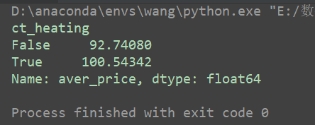
7.北方集中供暖对价格的影响

data['ct_heating'] = data['house_tag'].str.contains('集中供暖')ret = data[data['city'] =='北京'].groupby('ct_heating')['aver_price'].mean()
print(ret)

8.北上广深租房时都看重什么？

def layout_top3(city, data):layout_data = data[data['city'] == city]['layout'].value_counts().nlargest(3)bar = Bar(city+"最受欢迎的户型", width=600)bar.add("", layout_data.index, layout_data.values,legend_text_size=18, xaxis_label_textsize=14, yaxis_label_textsize=18,yaxis_min=8, legend_top=30, is_label_show=True)bar.render('beijing.html')return barlayout_top3('北京', data)

# 制作词云
from pyecharts import WordCloudbj_tag = []
for st in data[data['city']=='北京'].dropna(subset=['house_tag'])['house_tag']:bj_tag.extend(st.split(' '))ciyun = pd.Series(bj_tag)
ciyun = ciyun.value_counts()name, value = ciyun.index, ciyun.values
wordcloud = WordCloud(width=500, height=500)
wordcloud.add("", name, value, word_size_range=[20, 100])
wordcloud.render('ciyun.html')

9.各城市房屋出租销售比

没太看懂这块的想法

zs_ratio = [57036, 62779, 32039, 56758]/(data.groupby('city')['rent_price_listing'].sum()/data.groupby('city')['rent_area'].sum())/12
print(zs_ratio)
bar = Bar("各城市房屋租售比(租多少年可以在该城市买下一套房)", width=450)
bar.add("", zs_ratio.index, np.round(zs_ratio.values, 0),legend_text_size=18,xaxis_label_textsize=14,yaxis_label_textsize=18,yaxis_min=8, legend_top=30, is_label_show=True)
bar.render()