Ceres-Solver 官网教程翻译与学习

ceres-solver 参考1这是一个系列教程
ceres-solver 参考2这是一个入门教程
官网教程 推荐

仿函数（预备知识）

仿函数 参考
ceres当中代价函数（cost function）的构建当中用到了仿函数（functor），使用方法是在costfunction函数中重载了（）运算符（operator）
示例程序：

class Functor 
{
private:char* ss;int count;
public:explicit Functor(char* str) :ss(str),count(0){std::cout << "Functor: " << ss << "\n"; }void operator() (std::string str)  {count++;std::cout << "The Functor is called " << count << " times " <<str<< "\n";}
};
int main()
{Functor functor("construct");functor("first");functor("second");Functor functor1("construct1");functor1("first1");functor1("second1");
}

结果：

Functor: construct
The Functor is called 1 times first
The Functor is called 2 times second
Functor: construct1
The Functor is called 1 times first1
The Functor is called 2 times second1

Ceres

ceres用来解决边界约束鲁棒非线性最小二乘 问题 （bounds constrained robustified non-linear least squares problems）

最小二乘问题

边界约束非线性最小二成问题

$$\begin{array}{rl}\underset{x}{\min }& \frac{1}{2}\sum _i{\rho }_i(\Vert f_i(x_{i1},\dots ,x_{ik}){\Vert }^2)\\ \mathrm{s}.\mathrm{t}.& l_j\le x_j\le u_j\end{array}\text{\hspace{1em}(1)}$$

• 目标函数$\underset{x}{\min }f(x)$表示使$f(x)$最小的$x$取值
• 约束条件 $\mathrm{s}.\mathrm{t}.$是subject to 的简写

1. ${\rho }_i(\Vert f_i(x_{i1},\dots ,x_{ik}){\Vert }^2)$ 称为残差块(ResidualBlock)
2. $f_i(\cdot )$称为代价函数(CostFuction)
3. $[x_{i1},\dots ,x_{ik}]$称为参数块(ParameterBlock) 其中$x_{ik}$是标量(Scalar),参数块可以是一个标量群，也可以是单个标量
4. $l_j$, $u_j$是参数块(Parameter Block) $x_j$的边界条件
5. ${\rho }_i$称为损失函数(LossFunction) 是一个标量函数(Scalar Function)，用来减小异常值（outliers）对结果的非线性最小二乘求解结果的影响。当${\rho }_i(f_i(x_i))=f_i(x_i)$且$l_i=-\infty$, $u_i=\infty$时，我们就得到通常意义上的非线性最小二乘问题
   $$\frac{1}{2}\sum _i\Vert f(x_{i1},\dots ,x_{ik}){\Vert }^2\text{\hspace{1em}(2)}$$

Hello World

首先从一个查找函数最小值的问题起步
$$\frac{1}{2}(10-x{)}^2$$
这是一个很简单的问题，很容易得到最小值在$x=10$处，但是这是一个很好的起点来说明使用Ceres来解决问题的基本用法。
首先写一个仿函数（functor）来评价函数
$$f(x)=10-x$$

struct CostFunctor
{template <typename T>bool operator() (const T* const x, T* residual) const{residual[0] = 10.0 - x[0];return true;}
};

operator()是模板方法(Template Method)，这种方法假设输入与输出都是某个类型T，模板的使用允许ceres按照下面两种方法调用CostFunctor::operator()：

1. 当只需要计算残差值时T=double
2. 当需要Jacobian矩阵时T=Jet，Jet是Ceres定义的一个特殊类型
   一旦我们有办法计算残差方程(Residual Function)，是时候构建一个非线性最小二乘问题(non-linear least squares problem)并利用Ceres来求解

void TestCeres()
{ceres::Problem problem;double initial_x = 5.0;double x = initial_x;//建立唯一的代价函数（cost function）也可以称为 残差（residual）//Auto-Differentiation用来获得微分(derivative	)或者 Jacobian矩阵ceres::CostFunction* cost_function =new ceres::AutoDiffCostFunction<CostFunctor, 1, 1>(new CostFunctor);problem.AddResidualBlock(cost_function, nullptr, &x);//run the solver!ceres::Solver::Options options;options.linear_solver_type = ceres::DENSE_QR;options.minimizer_progress_to_stdout = true;ceres::Solver::Summary summary;ceres::Solve(options, &problem, &summary);std::cout << summary.BriefReport() << "\n";std::cout << "x : " << initial_x << " -> " << x << "\n";
}

AutoDiffCostFucntion将 CostFunctor的一个实例地址作为输入，自动的对其进行微分，并赋予其一个 CostFunction接口
结果: 我的结果跟官网的结果稍有不同，我的目标值（cost）比官网小，不知道为什么

iter      cost      cost_change  |gradient|   |step|    tr_ratio  tr_radius  ls_iter  iter_time  total_time0  1.250000e+01    0.00e+00    5.00e+00   0.00e+00   0.00e+00  1.00e+04        0    8.90e-04    1.96e-031  1.249750e-07    1.25e+01    5.00e-04   5.00e+00   1.00e+00  3.00e+04        1    1.18e-03    7.61e-032  1.388518e-16    1.25e-07    1.67e-08   5.00e-04   1.00e+00  9.00e+04        1    3.60e-04    8.09e-03
Ceres Solver Report: Iterations: 3, Initial cost: 1.250000e+01, Final cost: 1.388518e-16, Termination: CONVERGENCE
x : 5 -> 10

从$x=5$开始，求解器（solver）经过两次迭代得到最终结果10，仔细的读者应该发现这是一个线性问题，采用线性求解器应该就会求得优化结果。求解器的默认配置是面向非线性问题的，为了简化过程例子中并没有修改配置。使用Ceres-Solver确实有可能通过一次迭代得到这个问题的结果，在讲到Ceres收敛与参数设置时我们会详细的讨论这个问题。

导数（derivatives）

参考
导数与微分
Ceres-Solver与大多数优化包一样，依赖于能够在任意参数下评估（evaluate）目标函数中每一项的函数值与导数，能够正确并有效的做到这一点对获得好的结果至关重要。Ceres Solver提供了几种不同方法，在上面的例子中你已经见到了其中的一种-Automatic Differentiation（自动微分），我们现在考虑其他两种可能性（possibilities）：解析求导（Analytic Derivatives）与数值求导（Numerical Derivatives）

数值微分（Numerical Derivatives）

在某些情况下，我们无法定义一个模板代价函数，比如计算残差（residual）时调用了一个无法控制的库函数，这种情况下就可以使用数值求导。用户定义一个仿函数（functor）来计算残差（residual），并构建一个NumericDiffCostFunction，以f(x)=10-x为例，对应的仿函数（functor）为：

struct NumericalDiffCostFunctor
{bool operator()(const double* const x, double* residual) const{residual[0] = 10.0 - x[0];return true;}
};

按照如下方法加入Problem中

void TestCeresNumerical()
{ceres::Problem problem;double initial_x = 5;double x = initial_x;ceres::CostFunction* cost_function =new ceres::NumericDiffCostFunction<NumericalDiffCostFunctor, ceres::CENTRAL, 1, 1>(new NumericalDiffCostFunctor);problem.AddResidualBlock(cost_function, nullptr, &x);ceres::Solver::Options option;option.linear_solver_type = ceres::DENSE_QR;option.minimizer_progress_to_stdout = true;ceres::Solver::Summary summary;ceres::Solve(option, &problem, &summary);std::cout << summary.BriefReport() << "\n";std::cout << "x: " << initial_x << " -> " << x << "\n";
}

与Automatic Differentiation中我们使用的代码做对比

	ceres::CostFunction* cost_function =new ceres::AutoDiffCostFunction<CostFunctor, 1, 1>(new CostFunctor);problem.AddResidualBlock(cost_function, nullptr, &x);

与 Automatic Differentiation中的代码结构几乎一样（identical），但是增加了一个额外的参数ceres::CENTRAL用来表明采用哪种有限差分方案来计算数值导数。ceres::CENTRAL定义如下：NumericDiffCostFunction

enum NumericDiffMethodType {// Compute central finite difference: f'(x) ~ (f(x+h) - f(x-h)) / 2h.CENTRAL,// Compute forward finite difference: f'(x) ~ (f(x+h) - f(x)) / h.FORWARD,// Adaptive numerical differentiation using Ridders' method. Provides more// accurate and robust derivatives at the expense of additional cost// function evaluations.RIDDERS
};

总的来说我们推荐自动微分（Automatic Differentiation）来取代数值微分（Numerical Differentiation）。C++的模板类让自动微分十分高效，而数值微分计算量大，容易产生数值误差（numeric error），并且收敛（convergence）更慢。

解析法求导（Analytic Derivative）

有些情况下可能无法使用自动微分。比如，在某些情况下使用封闭解比自动微分中使用的链式法则（chain rule）的计算导数更有效。
在这种情况下，需要提供你自己的残差（residual）与 雅可比（Jacobian）计算代码。 定义一个CostFunction的子类（subclass）,如果你知道参数（parameter）与残差（residual）在编译时的大小也可以定义SizedCostFunction的子类。下面以实现$f(x)=10-x$的SimpleCostFunction为例

class QuadraticCostFunction : public ceres::SizedCostFunction<1, 1>
{
public:virtual ~QuadraticCostFunction() {}virtual bool Evaluate(double const* const* parameters,double* residuals,double** jacobians) const{const double x = parameters[0][0];residuals[0] = 10 - x;//compute the Jacobian if asked forif (jacobians != nullptr && jacobians[0] != nullptr){jacobians[0][0] = -1;}return true;}
};

下面是我自己写的，教程中没有

void testQuadraticCostFunction()
{ceres::Problem problem;double initial_x = 5;double x = initial_x;ceres::CostFunction* cost_function = new QuadraticCostFunction;problem.AddResidualBlock(cost_function,nullptr,&x);ceres::Solver::Options option;option.linear_solver_type = ceres::DENSE_QR;option.minimizer_progress_to_stdout = true;ceres::Solver::Summary summary;ceres::Solve(option, &problem, &summary);std::cout << summary.BriefReport() << "\n";std::cout << "x: " << initial_x << " -> " << x << '\n';
}

这里代码应该是写错了,将SimpleCOstFunction写成了QuadraticCostFunction
QuadraticCostFunction::Evaluate有一个参数（parameter）数组，一个输出的残差（residual）数组，和一个输出的雅可比（Jacobian）数组，雅可比数组是可选的，evaluate函数会检查jacobians是否为非空（non-null），如果是非空的就填入残差方程的导数值（value of the derivative of residual function）。在本例当中残差方程是线性的，所以雅可比矩阵是常数（constant）
从上面的例子中我们可以看出，实现CostFunction对象的过程有些枯燥，除非你有非常好的理由自己实现Jacobian矩阵，否则我们还是推荐你使用自动微分或者数值微分来构建残差块（residual blocks）
计算导数目前为止是使用Ceres最复杂的部分，根据情况使用者可能需要更复杂的导数计算方法。这一部分只是浅显的介绍了如何向Ceres提供导数，一旦你适应了使用NumericDiffCostFunctionandAutoDiffCostFunction，我们建议看一看DynamicAutoDiffCostFunction, CostFunctionToFunctor, NumericDiffFunctorandConditionedCostFunction来获取更多构建与计算代价函数的方法。

Powell’s Function

鲍威尔方程
现在考虑一个稍微复杂点的例子—鲍威尔方程的最小化，令$x=[x_1,x_2,x_3,x_4]$
$$\begin{array}{rl}{f}_1(x)& =x_1+10x_2\\ f_2(x)& =\sqrt{5}(x_3-x_4)\\ f_3(x)& =(x_2-2x_3{)}^2\\ f_4(x)& =\sqrt{10}(x_1-x_4{)}^2\\ F(x)& =[f_1(x),f_2(x),f_3(x),f_4(x)]\end{array}$$
$F(x)$是一个拥有四个参数，四组残差的方程，我们希望找到一个令 $\frac{1}{2}\Vert F(x){\Vert }^2$最小化的$x$
第一步，目标函数中的每一项都定义仿函数，下面是$f_1(x_1,x_2)$, $f_2(x_3,x_4)$, $f_3(x_2,x_3)$, $f_4(x_1,x_4)$的代码

struct F1
{template <typename T>bool operator()(const T* const x1, const T* const x2, T* residual) const{residual[0] = x1[0] + 10 * x2[0];return true;}
};
struct F2
{template <typename T>bool operator()(const T* const x3, const T* const x4, T* residual) const{residual[0] = sqrt(5) * (x3[0] - x4[0]);}
};
struct F3
{template <typename T>bool operator()(const T* const x2, const T* const x3, T* residual) const{residual[0] = (x2[0] - 2 * x3[0]) * (x2[0] - 2 * x3[0]);}
};
struct F4 
{template <typename T>bool operator()(const T* const x1, const T* const x4, T* residual)const{residual = sqrt(10.0) * (x1[0] - x4[0]) * (x1[0] - x4[0]);return true;}
};

利用上面定义的结构体按如下方法构建problem：

	double x1 = 3.0; double x2 = -1.0; double x3 = 0.0; double x4 = 1.0;ceres::Problem problem;problem.AddResidualBlock(new ceres::AutoDiffCostFunction<F1, 1, 1, 1>(new F1), nullptr, &x1, &x2);problem.AddResidualBlock(new ceres::AutoDiffCostFunction<F2, 1, 1, 1>(new F2), nullptr, &x3, &x4);problem.AddResidualBlock(new ceres::AutoDiffCostFunction<F3, 1, 1, 1>(new F3), nullptr, &x2, &x3);problem.AddResidualBlock(new ceres::AutoDiffCostFunction<F4, 1, 1, 1>(new F4), nullptr, &x1, &x4);ceres::Solver::Summary summary;ceres::Solver::Options option;option.max_num_iterations = 100;option.linear_solver_type = ceres::DENSE_QR;option.minimizer_progress_to_stdout = true;ceres::Solve(option, &problem, &summary);std::cout << "Initial: " << "x1 =" << x1 << ", x2= " << x2 << ", x3= " << x3 << ", x4= " << x4 << '\n';std::cout << summary.FullReport() << '\n';std::cout << "Final: " << "x1 =" << x1 << ", x2= " << x2 << ", x3= " << x3 << ", x4= " << x4 << '\n';

注意到每一个ResidualBlock只依赖两个参数，相应的残差对象也不依赖所有的四个参数。结果略。

Curve Fitting

到目前为止我们所见到的例子都是无数据的简单优化问题。最小方差与非线性最小方差分析的最初目的是对数据进行曲线拟合。现在正适合我们考虑这个问题。问题包含从曲线$e^{0.3x+0.1}$采样的数据，并向数据添加带有标准差（standard deviation）$\sigma =2$的高斯（Gaussian）噪声。现在我们用数据拟合曲线$$y=e^{mx+c}$$
我们先来定义一个模板类来计算残差。对每一个观测（observation）都有一个残差。

struct ExponentialResidual
{ExponentialResidual(double x, double y) :x_(x), y_(y) {}template <typename T>bool operator()(const T* const m, const T* const c, T* residual) const{residual[0] = y_ - exp(m[0] * x_ + c[0]);return ture;}
private:const double x_;const double y_;
};

假设观测数据存在一个$2n$大小的数组data当中, problem 的构建就是简单的对每一个观测数据创建一个CostFunction。

    const int kNumObservations = 67;// clang-format offconst double data[] = {  0.000000e+00, 1.133898e+00,
... }；//这里有67组数 一组有一个x，一个ydouble m = 0.0;double c = 0.0;ceres::Problem problem;for (int i = 0; i <kNumObservations; i++){ceres::CostFunction* cost_function =new ceres::AutoDiffCostFunction<ExponentialResidual, 1, 1, 1>(new ExponentialResidual(data[2 * i], data[2 * i + 1]));problem.AddResidualBlock(cost_function, nullptr, &m, &c);}ceres::Solver::Options option;option.max_num_iterations = 100;option.linear_solver_type = ceres::DENSE_QR;option.minimizer_progress_to_stdout = true;ceres::Solver::Summary summary;ceres::Solve(option, &problem, &summary);std::cout << summary.BriefReport() << '\n';std::cout << "Initial m: " << 0.0 << " c: " << 0.0 << '\n';std::cout << "Final   m: " << m << " c: " << c << '\n';

iter      cost      cost_change  |gradient|   |step|    tr_ratio  tr_radius  ls_iter  iter_time  total_time0  1.211734e+02    0.00e+00    3.61e+02   0.00e+00   0.00e+00  1.00e+04        0    1.80e-03    2.13e-031  2.334822e+03   -2.21e+03    3.61e+02   7.52e-01  -1.87e+01  5.00e+03        1    8.37e-04    3.48e-032  2.331438e+03   -2.21e+03    3.61e+02   7.51e-01  -1.86e+01  1.25e+03        1    4.32e-04    4.01e-033  2.311313e+03   -2.19e+03    3.61e+02   7.48e-01  -1.85e+01  1.56e+02        1    4.24e-04    4.52e-034  2.137268e+03   -2.02e+03    3.61e+02   7.22e-01  -1.70e+01  9.77e+00        1    4.26e-04    5.02e-035  8.553131e+02   -7.34e+02    3.61e+02   5.78e-01  -6.32e+00  3.05e-01        1    4.28e-04    5.54e-036  3.306595e+01    8.81e+01    4.10e+02   3.18e-01   1.37e+00  9.16e-01        1    2.11e-03    7.77e-037  6.426770e+00    2.66e+01    1.81e+02   1.29e-01   1.10e+00  2.75e+00        1    2.01e-03    9.90e-038  3.344546e+00    3.08e+00    5.51e+01   3.05e-02   1.03e+00  8.24e+00        1    2.24e-03    1.22e-029  1.987485e+00    1.36e+00    2.33e+01   8.87e-02   9.94e-01  2.47e+01        1    2.01e-03    1.44e-0210  1.211585e+00    7.76e-01    8.22e+00   1.05e-01   9.89e-01  7.42e+01        1    2.38e-03    1.69e-0211  1.063265e+00    1.48e-01    1.44e+00   6.06e-02   9.97e-01  2.22e+02        1    2.05e-03    1.91e-0212  1.056795e+00    6.47e-03    1.18e-01   1.47e-02   1.00e+00  6.67e+02        1    2.02e-03    2.12e-0213  1.056751e+00    4.39e-05    3.79e-03   1.28e-03   1.00e+00  2.00e+03        1    2.02e-03    2.34e-02
Ceres Solver Report: Iterations: 14, Initial cost: 1.211734e+02, Final cost: 1.056751e+00, Termination: CONVERGENCE
Initial m: 0 c: 0
Final   m:0.291861 c: 0.131439

从参数值$m=0$, $c=0$开始，初始的目标函数值是121.173。Ceres找到了一组结果$m=0.291861,c=0.131439$对应的目标函数值是1.05675。这些值与原始的模型参数 $y=e^{0.3x+0.1}$ 稍有不同，但是这个是可以预料到的。当从有噪声的数据中拟合曲线时，我们希望看到这个偏差（deviation）

Rubust Curve Fitting 鲁棒曲线拟合

如果假设数据中有一些离群值（outlier），也就是说有一些点不符合噪声模式，如果我们使用上面的代码来拟合这样的数据就会得到下面的曲线（摘自官网），注意拟合的曲线如何偏离真值。

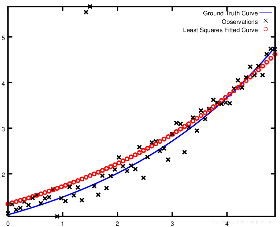
为了处理离群值outlier，标准的方法是利用损失函数LossFunction, 损失函数减小了交大残差对残差块的影响，通常较大残差是由离群值影响的。为了使一个损失函数与残差块关联起来，我们将

problem.AddResidualBlock(Cost_function, nullptr, &m, &c)

替换为

problem.AddResidualBlock(const_function, new CauchyLoss(0.5), &m, &c);

CauchyLoss是Ceres Solver的的一个损失函数。参数0.5制定了损失函数的幅度。这样就可以得到下面的较好结果：略

Bundle Adjustment

光束平差法1
光束平差法2 推荐
李群和李代数
自然常数$e$,工程中的自然数$1$
编写Ceres的一个重要原因是我们需要解决大规模的光束平差问题。
给出一组测量的图像特征坐标和其他相应数据，光束平差法的目标是找到使重投影误差最小的3D点坐标和相机参数。这个优化问题通常被规划为非线性最小方差问题，其中误差是观测道德特征坐标与相应3D点在相机相平面投影之间的$L_2$范数normal的平方square。Ceres 广泛的支持光束平差问题。

Reference
$L_0$范数：向量中非0元素的个数
$L_1$范数：向量中各个元素绝对值之和 $\Vert x{\Vert }_1=|x_1|+|x_2|+\cdots +|x_n|$
$L_2$范数：向量各元素平方和后求平方根 $\Vert x_2{\Vert }_2=\sqrt{|x_1{|}^2+|x_2{|}^2+\cdots +|x_n{|}^2}$

让我们来求解BAL数据集
此处未完待续

On Derivatives

Spivak Notation (斯皮瓦克标记法)

Michael Spivak – 微分几何的数学家
为了保持集体理智，我们使用Spivak关于导数的解释。这是一个实用的解释，使包含导数的表达式理解起来变得简单易懂
对于一个单变量的函数$f$,$f(a)$代表它再$a$点的值，$Df$代表它的一次导数，$Df(a)$是在$a$点的导数，也就是：$$Df(a)=\frac{d}{dx}f(x){|}_{x=a}$$
$D^k$代表$f$的第$k^{th}$次导数。
对于一个二元函数$g(x,y)$. $D_{1g}$与$D_{2g}$分别代表$g$的第一变量与第二变量的偏微分. 与经典标记法等效：
$$\begin{gathered} D_{1g}=\frac{\partial }{\partial x}g(x,y) \\ {D}_{2g}=\frac{\partial }{\partial y}g(x,y) \end{gathered}$$
$D_g$代表$g$的Jacobian矩阵：
$$D_g=[D_{1g},D_{2g}]$$
对于一个多变量函数$g:{\mathbb{R}}^n\to {\mathbb{R}}^m$, $D_g$ 代表$m\times n$的Jacobian矩阵. $D_{ig}$是$g$的第$i$个坐标的偏微分，是$D_g$的第$i$列。
最后，$D_1^{2}g$,$D_1{D}_{2}g$代表高阶偏微分。
For more see Michael Spivak’s book Calculus on Manifolds

Analytic Derivatives

考虑下面这个将曲线拟合到数据上的问题:
$$\frac{b_1}{(1+e^{b_2-b_3{x}_1}{)}^{1/b_4}}$$
也就是说给定一些数据 { x i , y i } , ∀ i = 1 , 2 , … , n \{x_i,y_i\},\forall{i}=1,2,\dots,n {xi​,yi​},∀i=1,2,…,n, 确定最适合数据的参数$b_1,b_2,b_3,b_4$。
这个问题也就是找到使下面目标函数最小的参数$b_1,b_2,b_3,b_4$
$$\begin{array}{rl}E(b_1,b_2,b_3,b_4)& =\sum _{i=1}^n{f}^2(b_1,b_2,b_3,b_4;x_i,y_j)\\ & =\sum _{i=1}^n(\frac{b_1}{(1+E^{b_2-b_3{x}_1})}-y_i{)}^2\end{array}$$
利用Ceres解决这个问题，我们需要定义一个代价函数来计算给定$x$与$y$关于$b_1,b_2,b_3,b_4$的残差Residual$f$和导数.
使用初级微积分，我们可以得到：
$$\begin{array}{rl}{D}_{1}f(b_1,b_2,b_3,b_4;x,y)& =\frac{1}{(1+e^{b_2-b_{3}x}{)}^{1/b_4}}\\ D_{2}f(b_1,b_2,b_3,b_4;x,y)& =\frac{-b_1{e}^{b2-b_{3}x}}{b_4(1+e^{b_2-b_{3}x}{)}^{1/b_4+1}}\\ D_{3}f(b_1,b_2,b_3,b_4;x,y)& =\frac{b_{1}x{e}^{b_2-b_{3}x}}{b_4(1+e^{b_2-b_{3}x}{)}^{1/b_4+1}}\\ D_{4}f(b_1,b_2,b_3,b_4;x,y)& =\frac{b_1\log (1+e^{b_2-b_{3}x})}{b_4^2(1+e^{b_2-b_{3}x}{)}^{1/b_4}}\end{array}$$

Tat43AnalyticOptimized比Rat43Analytic快了2.8倍。这种运行时的差异十分普遍。为了获得解析导数的最佳性能，需要对通用子表达式进行优化。

什么时候需要使用解析微分？

• 1、表达式简
• 单，例如线性的
• 2、一个计算机代数软件像Maple, Mathematica, SymPy可以用来对目标函数计算符号微分，并生成C++代码。
• 3、对效率要求极高，可以利用一些代数结构来获得比自动微分更好的性能。
  也就是说为了获得更好的性能，需要做大量的复杂工作。在走这条路之前， 评估计算Jacobian矩阵在整个求解过程中所占的时间非常有必要。记住Amdahl’s Law对你很有帮助。
• 4、没有其他方法计算导数，例如要计算下面这个多项式Polyomial根关于$x$, $y$的导数：
  $$a_3(x,y)z^3+a_2(x,y)z^2+a_1(x,y)z+a_0(x,y)=0$$
  这个方程的导数求解需要使用Inverse Function Theorem
• 5、你就是喜欢手动计算导数。

附注Footnotes

最佳拟合的概念依赖用于评价拟合质量目标函数的选择，目标函数反过来也依赖于产生观测的基本噪声处理。当噪声是高斯噪声时，最小化方差和是正确的方法。在这种情况下，参数的优化值是极大似然估计

Numeric Derivatives

Forward Differences

Central Differences

Ridders’ Methord

Automatic Derivatives

Interfacing With Automatic Differentiation

Reference
当代价函数是一个明确的表达式时，可以直接使用自动微分。但是并不总是这样，有时代价函数需要与外部程序或数据进行交互。在这一章中我们考虑几种不同的方法。
我们考虑下面这个问题，通过查找参数$\theta$与$t$来优化下面这个优化问题：
$$\begin{array}{rl}\min & \sum \Vert y_i-f(\Vert q_i{\Vert }^2)q_i{\Vert }^2\\ \mathrm{s}\mathrm{u}\mathrm{c}\mathrm{h}\mathrm{t}\mathrm{h}\mathrm{a}\mathrm{t}& q_i=R(\theta )x_i+t\end{array}$$
这里$R$是一个二维的旋转矩阵，使用$\theta$进行参数化。$t$是一个二维向量。$f$是一个外部的畸变函数distortion function
先考虑这个情况，首先有一个模板函数TemplatedComputeDistortion来计算函数$f$。那么对应的残差仿函数就很简单，如下所示：

template <typename T> T TemplatedComputeDistortion(const T r2) {const double k1 = 0.0082;const double k2 = 0.000023;return 1.0 + k1 * y2 + k2 * r2 * r2;//此处y2 应为 r2
}struct Affine2DWithDistortion {Affine2DWithDistortion(const double x_in[2], const double y_in[2]) {x[0] = x_in[0];x[1] = x_in[1];y[0] = y_in[0];y[1] = y_in[1];}template <typename T>bool operator()(const T* theta,const T* t,T* residuals) const {const T q_0 =  cos(theta[0]) * x[0] - sin(theta[0]) * x[1] + t[0];const T q_1 =  sin(theta[0]) * x[0] + cos(theta[0]) * x[1] + t[1];const T f = TemplatedComputeDistortion(q_0 * q_0 + q_1 * q_1); // !!!residuals[0] = y[0] - f * q_0;residuals[1] = y[1] - f * q_1;return true;}double x[2];double y[2];
};

现在我们考虑三种不能直接应用自动微分的$f$:

• 1.非模板函数
• 2.计算自身值与导数的函数
• 3.函数被定义成一个插值的函数表
  下面依次考虑这三种情况.

A function that return its value(返回值的非模板函数)

假设给定一个方程ComputeDistortionValue声明signature如下

double ComputeDistortionValue(double r2)

这个函数计算了$f$的值，函数内部的实现不重要，将这个函数与Affine2DWithDistortion对接总共分三步：

• 1、将ComputeDistortionValue封装warp成仿函数ComputeDistortionValueFunctor
• 2、对ComputeDistortionValueFunctor使用’NumericDiffCostFunction’进行数值微分
• 3、使用CostFunctionToFunctor对CostFunction对象进行封装，得到一个含有模板函数Operator()的仿函数对象，这个仿函数对象将NumericDiffCostFunction计算的Jacobian矩阵传送到Jet对象中

struct ComputeDistortionValueFunctor {bool operator()(const double* r2, double* value) const {*value = ComputeDistortionValue(r2[0]);return true;}
};struct Affine2DWithDistortion {Affine2DWithDistortion(const double x_in[2], const double y_in[2]) {x[0] = x_in[0];x[1] = x_in[1];y[0] = y_in[0];y[1] = y_in[1];compute_distortion.reset(new ceres::CostFunctionToFunctor<1, 1>(new ceres::NumericDiffCostFunction<ComputeDistortionValueFunctor,ceres::CENTRAL,1,1>(new ComputeDistortionValueFunctor)));}template <typename T>bool operator()(const T* theta, const T* t, T* residuals) const {const T q_0 = cos(theta[0]) * x[0] - sin(theta[0]) * x[1] + t[0];const T q_1 = sin(theta[0]) * x[0] + cos(theta[0]) * x[1] + t[1];const T r2 = q_0 * q_0 + q_1 * q_1;T f;(*compute_distortion)(&r2, &f);residuals[0] = y[0] - f * q_0;residuals[1] = y[1] - f * q_1;return true;}double x[2];double y[2];std::unique_ptr<ceres::CostFunctionToFunctor<1, 1> > compute_distortion;
};

---

未完待续