tensorflow入门教程(三十五)facenet源码分析之MTCNN--人脸检测及关键点检测

本文主要是介绍tensorflow入门教程(三十五)facenet源码分析之MTCNN--人脸检测及关键点检测，希望对大家解决编程问题提供一定的参考价值，需要的开发者们随着小编来一起学习吧！

#
#作者：韦访
#博客：https://blog.csdn.net/rookie_wei
#微信：1007895847
#添加微信的备注一下是CSDN的
#欢迎大家一起学习
#

------韦访 20190123

1、概述

上一讲提到使用MTCNN可以将人脸检测出来，并且识别出5个关键点（左眼、右眼、鼻子、左嘴角、右嘴角）的位置。这一讲我们来分析一个facenet的源码，作为人脸识别的三讲的一个补充。下面的内容配合人脸识别（上、中、下）那三讲来看，链接地址如下：https://blog.csdn.net/rookie_wei/article/details/81676177

https://blog.csdn.net/rookie_wei/article/details/82078373

https://blog.csdn.net/rookie_wei/article/details/82085152

2、准备工作

首先，下载LFW数据集，下载链接为，

http://vis-www.cs.umass.edu/lfw/lfw.tgz

然后，下载FaceNet源码，下载链接，

https://codeload.github.com/davidsandberg/facenet/zip/master

项目的GitHub链接为，

https://github.com/davidsandberg/facenet/tree/master

FaceNet源码下载完后，解压，然后，将LFW数据集解压到FaceNet源码的根目录下，结构如下，

FaceNet源码的结构和环境搭建等，请看人脸识别（中）那讲，这里就不赘述。一切准就绪以后，执行以下代码就开始进行人脸检测，

python src/align/align_dataset_mtcnn.py lfw lfw_align_160 --image_size 160 --margin 32 --random_order

运行结果如下，

则表示开始进行人脸检测的工作了，运行结束后，lfw_align_160文件夹里有如下子文件夹， 

 每个文件夹里有截取好的人脸框，具体请看人脸识别（中）的内容，我们这讲的重点是源码分析。

3、main函数分析

根据上面的命令，我们先来看src/align/align_dataset_mtcnn.py文件，找到程序入口，

if __name__ == '__main__':main(parse_arguments(sys.argv[1:]))

parse_arguments函数是一些参数的设置和解析，不多说了，下面来看main函数有什么鬼。

def main(args):sleep(random.random())#如果还没有输出文件夹，则创建output_dir = os.path.expanduser(args.output_dir)if not os.path.exists(output_dir):os.makedirs(output_dir)#在日志目录的文本文件中存储一些Git修订信息# Store some git revision info in a text file in the log directorysrc_path,_ = os.path.split(os.path.realpath(__file__))#在output_dir文件夹下创建revision_info.txt文件，里面存的是执行该命令时的参数信息#当前使用的tensorflow版本，git hash,git difffacenet.store_revision_info(src_path, output_dir, ' '.join(sys.argv))# 获取数据集下所有人名和其人名目录下是所有图片，# 放到ImageClass类中，再将类存到dataset列表里dataset = facenet.get_dataset(args.input_dir)print('Creating networks and loading parameters')

上面的代码还是比较简单的，创建我们要存储的人脸图的文件夹，再写入一些环境信息，再加载FLW数据集到dataset。

with tf.Graph().as_default():#设置Session的GPU参数，每条线程分配多少显存gpu_options = tf.GPUOptions(per_process_gpu_memory_fraction=args.gpu_memory_fraction)sess = tf.Session(config=tf.ConfigProto(gpu_options=gpu_options, log_device_placement=False))with sess.as_default():#获取P-Net，R-Net，O-Net网络pnet, rnet, onet = align.detect_face.create_mtcnn(sess, None)

接着，就是加载P-Net、R-Net、O-Net网络，这里是比较核心的，我们稍后再分析，先把握全局。

minsize = 20 # minimum size of face
threshold = [ 0.6, 0.7, 0.7 ]  # three steps's threshold
factor = 0.709 # scale factor# Add a random key to the filename to allow alignment using multiple processes
# 获取一个随机数，用于创建下面的文件名
random_key = np.random.randint(0, high=99999)
# 将图片和求得的相应的Bbox保存到bounding_boxes_XXXXX.txt文件里
bounding_boxes_filename = os.path.join(output_dir, 'bounding_boxes_%05d.txt' % random_key)

然后是一些参数的设置，这些参数我们在获取人脸框中会用到。而bounding_boxes_filename文件则会存储每张图片的人脸框的数据，如下图所示，

每行数据的前面是人脸图片，后面的四个数据是人脸框的数据，分别对应与左上角和右下角相对于原始图片的的坐标。如果有需要，你也可以将关键点的坐标也存进来。

with open(bounding_boxes_filename, "w") as text_file:#处理图片的总数量nrof_images_total = 0nrof_successfully_aligned = 0#是否对所有图片进行洗牌if args.random_order:random.shuffle(dataset)for cls in dataset:output_class_dir = os.path.join(output_dir, cls.name)#如果目的文件夹里还没有相应的人名的文件夹，则创建相应文件夹if not os.path.exists(output_class_dir):os.makedirs(output_class_dir)if args.random_order:random.shuffle(cls.image_paths)for image_path in cls.image_paths:nrof_images_total += 1# 对齐后的图片文件名filename = os.path.splitext(os.path.split(image_path)[1])[0]output_filename = os.path.join(output_class_dir, filename+'.png')print(image_path)if not os.path.exists(output_filename):try:#读取图片文件img = misc.imread(image_path)except (IOError, ValueError, IndexError) as e:errorMessage = '{}: {}'.format(image_path, e)print(errorMessage)else:if img.ndim<2:print('Unable to align "%s"' % image_path)text_file.write('%s\n' % (output_filename))continueif img.ndim == 2:img = facenet.to_rgb(img)img = img[:,:,0:3]

上面是读取要进行处理的原始图片和获得人脸框后的图片的存储路径。不是很关键的信息，我们继续往下看。

#检测人脸，bounding_boxes可能包含多张人脸框数据，
# 一张人脸框有5个数据，第一和第二个数据表示框左上角坐标，第三个第四个数据表示框右下角坐标，
#最后一个数据应该是可信度
bounding_boxes, _ = align.detect_face.detect_face(img, minsize, pnet, rnet, onet, threshold, factor)
#获得的人脸数量
nrof_faces = bounding_boxes.shape[0]
if nrof_faces>0:det = bounding_boxes[:,0:4]det_arr = []#原图片大小img_size = np.asarray(img.shape)[0:2]if nrof_faces>1:if args.detect_multiple_faces:# 如果要检测多张人脸的话for i in range(nrof_faces):det_arr.append(np.squeeze(det[i]))else:#即使有多张人脸，也只要一张人脸就够了#获取人脸框的大小bounding_box_size = (det[:,2]-det[:,0])*(det[:,3]-det[:,1])#原图片中心坐标img_center = img_size / 2#求人脸框中心点相对于图片中心点的偏移，#(det[:,0]+det[:,2])/2和(det[:,1]+det[:,3])/2组成的坐标其实就是人脸框中心点offsets = np.vstack([ (det[:,0]+det[:,2])/2-img_center[1], (det[:,1]+det[:,3])/2-img_center[0] ])#求人脸框中心到图片中心偏移的平方和#假设offsets=[[   4.20016056  145.02849352 -134.53862838] [ -22.14250919  -26.74770141  -30.76835772]]#则offset_dist_squared=[  507.93206189 21748.70346425 19047.33436466]offset_dist_squared = np.sum(np.power(offsets,2.0),0)# 用人脸框像素大小减去偏移平方和的两倍，得到的结果哪个大就选哪个人脸框# 其实就是综合考虑了人脸框的位置和大小，优先选择框大，又靠近图片中心的人脸框index = np.argmax(bounding_box_size-offset_dist_squared*2.0) # some extra weight on the centeringdet_arr.append(det[index,:])else:#只有一个人脸框的话，那就没得选了det_arr.append(np.squeeze(det))

上面的align.detect_face.detect_face函数就是人脸检测的核心了，bounding_boxes里存的就是人脸框的数据，注意，这里可能包含多张人脸的数据。第二个返回值这里没有用到，所以用了“_”来接受，其实这个返回值也是很有用的，就是5个关键点的坐标。我们后面再详细分析。继续往下看，

for i, det in enumerate(det_arr):det = np.squeeze(det)bb = np.zeros(4, dtype=np.int32)#边界框周围的裁剪边缘，就是我们这里要裁剪的人脸框要比MTCNN获取的人脸框大一点，#至于大多少，就由margin参数决定了bb[0] = np.maximum(det[0]-args.margin/2, 0)bb[1] = np.maximum(det[1]-args.margin/2, 0)bb[2] = np.minimum(det[2]+args.margin/2, img_size[1])bb[3] = np.minimum(det[3]+args.margin/2, img_size[0])#裁剪人脸框，再缩放cropped = img[bb[1]:bb[3],bb[0]:bb[2],:]scaled = misc.imresize(cropped, (args.image_size, args.image_size), interp='bilinear')nrof_successfully_aligned += 1filename_base, file_extension = os.path.splitext(output_filename)if args.detect_multiple_faces:output_filename_n = "{}_{}{}".format(filename_base, i, file_extension)else:output_filename_n = "{}{}".format(filename_base, file_extension)#保存图片misc.imsave(output_filename_n, scaled)#记录信息到bounding_boxes_XXXXX.txt文件里text_file.write('%s %d %d %d %d\n' % (output_filename_n, bb[0], bb[1], bb[2], bb[3]))

这里就是获取人脸框数据以后，对原始图片的截取，这里截图的人脸框比上面获取的人脸框会大一点，这样才要做人脸识别嘛。最后，将人脸图片和对应的人脸框坐标存储到bounding_boxes_xxxxx.txt文件里。这就是FaceNet人脸检测的主框架，下面我们来具体分析。

4、P-Net、R-Net、O-Net网络定义

加载P-Net、R-Net、O-Net网络的函数是align.detect_face.create_mtcnn，我们看看它怎么实现的，该函数在src/align/detect_face.py文件里定义，

#创建MTCNN网络
#关于MTCNN网络，参考博客：https://blog.csdn.net/rookie_wei/article/details/81676177
def create_mtcnn(sess, model_path):if not model_path:model_path,_ = os.path.split(os.path.realpath(__file__))with tf.variable_scope('pnet'):#P-Net网络的输入，输入的宽高不限data = tf.placeholder(tf.float32, (None,None,None,3), 'input')pnet = PNet({'data':data})pnet.load(os.path.join(model_path, 'det1.npy'), sess)with tf.variable_scope('rnet'):# R-Net网络的输入是24*24*3data = tf.placeholder(tf.float32, (None,24,24,3), 'input')rnet = RNet({'data':data})rnet.load(os.path.join(model_path, 'det2.npy'), sess)with tf.variable_scope('onet'):# O-Net网络的输入是48*48*3data = tf.placeholder(tf.float32, (None,48,48,3), 'input')onet = ONet({'data':data})onet.load(os.path.join(model_path, 'det3.npy'), sess)#返回两个参数，第一个参数是人脸框，第二个参数是是否人脸的概率pnet_fun = lambda img : sess.run(('pnet/conv4-2/BiasAdd:0', 'pnet/prob1:0'), feed_dict={'pnet/input:0':img})# 返回两个参数，第一个参数是人脸框，第二个参数是是否人脸的概率rnet_fun = lambda img : sess.run(('rnet/conv5-2/conv5-2:0', 'rnet/prob1:0'), feed_dict={'rnet/input:0':img})# 返回三个参数，第一个参数是人脸框，第二个参数是是否人脸的概率，第三个参数是5个关键点坐标onet_fun = lambda img : sess.run(('onet/conv6-2/conv6-2:0', 'onet/conv6-3/conv6-3:0', 'onet/prob1:0'), feed_dict={'onet/input:0':img})return pnet_fun, rnet_fun, onet_fun

可以看到，该函数定义了3个占位符，大小依次是三个网络的输入图片的大小，第一个网络P-Net不需要指定输入图片大小，R-Net和O-Net网络输入大小分别是24*24*3和48*48*3。

我们先来看PNet是什么鬼，

#P-Net网络
class PNet(Network):def setup(self):(self.feed('data') #pylint: disable=no-value-for-parameter, no-member# 第一层卷积核大小为3*3，输出通道为10层.conv(3, 3, 10, 1, 1, padding='VALID', relu=False, name='conv1').prelu(name='PReLU1').max_pool(2, 2, 2, 2, name='pool1')# 第二层卷积核大小也为3*3，输出通道为16层.conv(3, 3, 16, 1, 1, padding='VALID', relu=False, name='conv2').prelu(name='PReLU2')# 第三层卷积核大小也为3*3，输出通道为32层.conv(3, 3, 32, 1, 1, padding='VALID', relu=False, name='conv3').prelu(name='PReLU3')# 这里应该就是face classification的输出.conv(1, 1, 2, 1, 1, relu=False, name='conv4-1').softmax(3,name='prob1'))#这里应该是bounding box regression的输出(self.feed('PReLU3') #pylint: disable=no-value-for-parameter.conv(1, 1, 4, 1, 1, relu=False, name='conv4-2'))

可以看到，PNet其实是一个类，这个类继承Network这个类，如果直接看它的setup函数，也能大概知道，这个函数其实是在构建一个神经网络，对比人脸识别（上）中介绍的P-Net网络的那张图，一看就明白了。我们还是先看Network这个类做了写什么吧，有其父必有其子嘛，所以，先去看父类。

class Network(object):def __init__(self, inputs, trainable=True):# The input nodes for this networkself.inputs = inputs# The current list of terminal nodesself.terminals = []# Mapping from layer names to layersself.layers = dict(inputs)# If true, the resulting variables are set as trainableself.trainable = trainable#设置神经网络，子类实现self.setup()#设置神经网络，由子类实现def setup(self):"""Construct the network. """raise NotImplementedError('Must be implemented by the subclass.')

先来看它的构造函数__init__，里面调用一个setup函数，而看这个类实现的setup函数可知，继承这个类的子类必须得实现这个setup函数，这就是我们看到的PNet类的setup函数，它的作用就是构造神经网络。所以，我猜RNet网络和ONet网络肯定也是实现setup函数来构造自己的网络的。

再看load函数，

#加载已经训练好的网络的weights数据
def load(self, data_path, session, ignore_missing=False):"""Load network weights.data_path: The path to the numpy-serialized network weightssession: The current TensorFlow sessionignore_missing: If true, serialized weights for missing layers are ignored."""data_dict = np.load(data_path, encoding='latin1').item() #pylint: disable=no-memberfor op_name in data_dict:with tf.variable_scope(op_name, reuse=True):for param_name, data in iteritems(data_dict[op_name]):try:var = tf.get_variable(param_name)session.run(var.assign(data))except ValueError:if not ignore_missing:raise

我们看它怎么用的，在create_mtcnn函数中看到它的用法如下，

pnet.load(os.path.join(model_path, 'det1.npy'), sess)
rnet.load(os.path.join(model_path, 'det2.npy'), sess)
onet.load(os.path.join(model_path, 'det3.npy'), sess)

传入一个文件和session，det1.npy、det2.npy、det3.npy分别对应于P-Net、R-Net、O-Net网络训练好的模型的参数，所以这个load函数就是导入这些参数，以使这三个网络能直接工作。

继续看，feed函数，

#通过替换终端节点为下一个操作设置输入。参数可以是层名称，也可以是实际层。
def feed(self, *args):"""Set the input(s) for the next operation by replacing the terminal nodes.The arguments can be either layer names or the actual layers."""assert len(args) != 0self.terminals = []for fed_layer in args:if isinstance(fed_layer, string_types):try:fed_layer = self.layers[fed_layer]except KeyError:raise KeyError('Unknown layer name fed: %s' % fed_layer)self.terminals.append(fed_layer)return self

我们也先看它怎么用，我们才更好的理解它，看PNet类的setup函数就有它的用法，

def setup(self):(self.feed('data') #pylint: disable=no-value-for-parameter, no-member# 第一层卷积核大小为3*3，输出通道为10层.conv(3, 3, 10, 1, 1, padding='VALID', relu=False, name='conv1').prelu(name='PReLU1').max_pool(2, 2, 2, 2, name='pool1')# 第二层卷积核大小也为3*3，输出通道为16层.conv(3, 3, 16, 1, 1, padding='VALID', relu=False, name='conv2').prelu(name='PReLU2')# 第三层卷积核大小也为3*3，输出通道为32层.conv(3, 3, 32, 1, 1, padding='VALID', relu=False, name='conv3').prelu(name='PReLU3')# 这里应该就是face classification的输出.conv(1, 1, 2, 1, 1, relu=False, name='conv4-1').softmax(3,name='prob1'))#这里应该是bounding box regression的输出(self.feed('PReLU3') #pylint: disable=no-value-for-parameter.conv(1, 1, 4, 1, 1, relu=False, name='conv4-2'))

先来看，

(self.feed('PReLU3') #pylint: disable=no-value-for-parameter.conv(1, 1, 4, 1, 1, relu=False, name='conv4-2'))

这里的PReLU3是上面网络定义的第三层网络的输出，再结合我们P-Net网络结构图来看，

第三层网络输出后，再经过一个1*1*4的卷积层，得到bounding box regression。所以这feed函数其实就是获取网络节点，想获取哪个网络节点就传入那个网络节点的名字即可，而self.feed('data')的data就是create_mtcnn函数中传入的占位符，也就是输入图片的数据。

再往下看，

#卷积层
@layer
def conv(self,inp,k_h,k_w,c_o,s_h,s_w,name,relu=True,padding='SAME',group=1,biased=True):# Verify that the padding is acceptableself.validate_padding(padding)# Get the number of channels in the inputc_i = int(inp.get_shape()[-1])# Verify that the grouping parameter is validassert c_i % group == 0assert c_o % group == 0# Convolution for a given input and kernelconvolve = lambda i, k: tf.nn.conv2d(i, k, [1, s_h, s_w, 1], padding=padding)with tf.variable_scope(name) as scope:kernel = self.make_var('weights', shape=[k_h, k_w, c_i // group, c_o])# This is the common-case. Convolve the input without any further complications.output = convolve(inp, kernel)# Add the biasesif biased:biases = self.make_var('biases', [c_o])output = tf.nn.bias_add(output, biases)if relu:# ReLU non-linearityoutput = tf.nn.relu(output, name=scope.name)return output#prelu激活函数
@layer
def prelu(self, inp, name):with tf.variable_scope(name):i = int(inp.get_shape()[-1])alpha = self.make_var('alpha', shape=(i,))output = tf.nn.relu(inp) + tf.multiply(alpha, -tf.nn.relu(-inp))return output#池化层
@layer
def max_pool(self, inp, k_h, k_w, s_h, s_w, name, padding='SAME'):self.validate_padding(padding)return tf.nn.max_pool(inp,ksize=[1, k_h, k_w, 1],strides=[1, s_h, s_w, 1],padding=padding,name=name)
#全连接层
@layer
def fc(self, inp, num_out, name, relu=True):with tf.variable_scope(name):input_shape = inp.get_shape()if input_shape.ndims == 4:# The input is spatial. Vectorize it first.dim = 1for d in input_shape[1:].as_list():dim *= int(d)feed_in = tf.reshape(inp, [-1, dim])else:feed_in, dim = (inp, input_shape[-1].value)weights = self.make_var('weights', shape=[dim, num_out])biases = self.make_var('biases', [num_out])op = tf.nn.relu_layer if relu else tf.nn.xw_plus_bfc = op(feed_in, weights, biases, name=name)return fc"""
Multi dimensional softmax,
refer to https://github.com/tensorflow/tensorflow/issues/210
compute softmax along the dimension of target
the native softmax only supports batch_size x dimension
"""
@layer
def softmax(self, target, axis, name=None):max_axis = tf.reduce_max(target, axis, keepdims=True)target_exp = tf.exp(target-max_axis)normalize = tf.reduce_sum(target_exp, axis, keepdims=True)softmax = tf.div(target_exp, normalize, name)return softmax

上面就是定义卷积层（conv）、激活函数（prelu）、池化层（max_pool）、全连接层（fc）、softmax函数的定义了，还有其他一些辅助的函数就不介绍了。R-Net、O-Net类类似，只是网络结构不同罢了，定义如下，

#R-Net网络
class RNet(Network):def setup(self):(self.feed('data') #pylint: disable=no-value-for-parameter, no-member#第一层卷积核大小为3*3，输出通道为28层.conv(3, 3, 28, 1, 1, padding='VALID', relu=False, name='conv1').prelu(name='prelu1').max_pool(3, 3, 2, 2, name='pool1')# 第二层卷积核大小为3*3，输出通道为48层.conv(3, 3, 48, 1, 1, padding='VALID', relu=False, name='conv2').prelu(name='prelu2').max_pool(3, 3, 2, 2, padding='VALID', name='pool2')# 第三层卷积核大小为2*2，输出通道为64层.conv(2, 2, 64, 1, 1, padding='VALID', relu=False, name='conv3').prelu(name='prelu3')# 第四层全连接网络，输出为128.fc(128, relu=False, name='conv4').prelu(name='prelu4')# 全连接层，这里是face classification的输出，输出为2.fc(2, relu=False, name='conv5-1').softmax(1,name='prob1'))# 全连接层，这里是bounding box regression的输出，输出为4(self.feed('prelu4') #pylint: disable=no-value-for-parameter.fc(4, relu=False, name='conv5-2'))
#O-Net网络
class ONet(Network):def setup(self):(self.feed('data') #pylint: disable=no-value-for-parameter, no-member# 第一层卷积核大小为3*3，输出通道为32层.conv(3, 3, 32, 1, 1, padding='VALID', relu=False, name='conv1').prelu(name='prelu1').max_pool(3, 3, 2, 2, name='pool1')# 第二层卷积核大小为3*3，输出通道为64层.conv(3, 3, 64, 1, 1, padding='VALID', relu=False, name='conv2').prelu(name='prelu2').max_pool(3, 3, 2, 2, padding='VALID', name='pool2')# 第三层卷积核大小为3*3，输出通道为64层.conv(3, 3, 64, 1, 1, padding='VALID', relu=False, name='conv3').prelu(name='prelu3').max_pool(2, 2, 2, 2, name='pool3')# 第四层卷积核大小为2*2，输出通道为128层.conv(2, 2, 128, 1, 1, padding='VALID', relu=False, name='conv4').prelu(name='prelu4')# 全连接层，输出为256.fc(256, relu=False, name='conv5').prelu(name='prelu5')# 全连接层，这里是face classification的输出，输出为2.fc(2, relu=False, name='conv6-1').softmax(1, name='prob1'))# 全连接层，这里是bounding box regression的输出，输出为4(self.feed('prelu5') #pylint: disable=no-value-for-parameter.fc(4, relu=False, name='conv6-2'))# 全连接层，这里是Facial landmark localization的输出，输出为10(self.feed('prelu5') #pylint: disable=no-value-for-parameter.fc(10, relu=False, name='conv6-3'))

以上就是P-Net、R-Net、O-Net网络的定义了。

5、detect_face函数之图像金字塔

人脸检测的函数是align.detect_face.detect_face，这个就是人脸检测的核心的难点了，该函数也在src/align/detect_face.py文件里定义，我们来看看。

#检测人脸，返回人脸框和五个关键点的坐标
def detect_face(img, minsize, pnet, rnet, onet, threshold, factor):"""Detects faces in an image, and returns bounding boxes and points for them.img: input imageminsize: minimum faces' sizepnet, rnet, onet: caffemodelthreshold: threshold=[th1, th2, th3], th1-3 are three steps's thresholdfactor: the factor used to create a scaling pyramid of face sizes to detect in the image."""factor_count=0total_boxes=np.empty((0,9))points=np.empty(0)#获取输入的图片的宽高h=img.shape[0]w=img.shape[1]#宽/高，谁小取谁minl=np.amin([h, w])m=12.0/minsizeminl=minl*m# create scale pyramid#创建比例金字塔scales=[]while minl>=12:scales += [m*np.power(factor, factor_count)]minl = minl*factorfactor_count += 1

首先是一些参数的初始化，还有创建金字塔比例，这个金字塔比例我们接着可视化的看看是怎么回事，

#将图片显示出来
# --韦访添加
plt.figure()
scale_img = img.copy()# first stage
#第一步，首先将图像缩放到不同尺寸形成“图像金字塔”
#然后，经过P-Net网络
for scale in scales:#宽高要取整hs=int(np.ceil(h*scale))ws=int(np.ceil(w*scale))#使用opencv的方法对图片进行缩放im_data = imresample(img, (hs, ws))#可视化的显示“图像金字塔”的效果# --韦访添加scale_img[0:im_data.shape[0], 0:im_data.shape[1]] = 0scale_img[0:im_data.shape[0], 0:im_data.shape[1]] = im_data[0:im_data.shape[0], 0:im_data.shape[1]]print('im_data.shape[0]', im_data.shape[0])print('im_data.shape[1]', im_data.shape[1])#对图片数据进行归一化处理im_data = (im_data-127.5)*0.0078125#增加一个维度，即batch size，因为我们这里每次只处理一张图片，其实batch size就是1img_x = np.expand_dims(im_data, 0)img_y = np.transpose(img_x, (0,2,1,3))# 送进P-Net网络# 假设img_y.shape=(1, 150, 150, 3)# 因为P-Net网络要经过3层核为3*3步长为1*1的卷积层，一层步长为2*2池化层# 所以conv4-2层输出形状为(1, 70, 70, 4)# 70是这么来的，(150-3+1)/1=148，经过池化层后为148/2=74，# 再经过一个卷积层(74-3+1)/1=72，再经过一个卷积层(72-3+1)/1=70# 计算方法参考博客：https://blog.csdn.net/rookie_wei/article/details/80146620# prob1层的输出形状为(1, 70, 70, 2)out = pnet(img_y)# 又变回来# out0的形状是(1, 70, 70, 4)# 返回的是可能是人脸的框的坐标out0 = np.transpose(out[0], (0,2,1,3))# out1的形状是(1, 70, 70, 2)# 返回的是对应与out0框中是人脸的可信度，第2个值为是人脸的概率out1 = np.transpose(out[1], (0,2,1,3))#out1[0,:,:,1]：表示框的可信度，只要一个值即可，因为这两个值相加严格等于1，这里只要获取“是”人脸框的概率#out0[0,:,:,:]：人脸框#scales:图片缩减比例#threshold:阈值，这里取0.6boxes, _ = generateBoundingBox(out1[0,:,:,1].copy(), out0[0,:,:,:].copy(), scale, threshold[0])# inter-scale nmspick = nms(boxes.copy(), 0.5, 'Union')if boxes.size>0 and pick.size>0:boxes = boxes[pick,:]total_boxes = np.append(total_boxes, boxes, axis=0)# --韦访添加
plt.imshow(scale_img)
plt.show()
exit()

先来看效果，随便删除lfw_align_160文件夹下的一个子文件夹，再执行以下命令，

python src/align/align_dataset_mtcnn.py lfw lfw_align_160 --image_size 160 --margin 32 --random_order

运行结果，

这样就可以对每个尺寸的图片通过神经网络计算一次，因为在原始图片中，人脸可能存在不同的尺寸，有个脸大，有的脸小。对于脸小的，可以在放大后的图片上检测，对于脸大的，可以在缩小后的图片上检测，这样就可以在统一的尺寸下检测人脸了。

6、P-Net

上面代码中，

out = pnet(img_y)

就是P-Net网络，out有两个值，第一个值out[0]是P-Net认为是人脸框的坐标，第二个值out[1]是P-Net认为out[0]是（或不是）人脸框的概率。

boxes, _ = generateBoundingBox(out1[0,:,:,1].copy(), out0[0,:,:,:].copy(), scale, threshold[0])

generateBoundingBox函数则根据out、scale（缩放比例）、threshold（可信度阈值，可信度大于该值才保留该人脸框）三个参数，初次筛选并还原人脸框尺寸，generateBoundingBox代码如下，

 

#imap：框是人脸的可信度
#reg：所有人脸框
#scale：图片缩减比例
#t：阈值
def generateBoundingBox(imap, reg, scale, t):"""Use heatmap to generate bounding boxes"""stride=2cellsize=12imap = np.transpose(imap)#获取x1,y1,x2,y2的坐标dx1 = np.transpose(reg[:,:,0])dy1 = np.transpose(reg[:,:,1])dx2 = np.transpose(reg[:,:,2])dy2 = np.transpose(reg[:,:,3])#获取可信度大于阈值的人脸框的坐标y, x = np.where(imap >= t)#只有一个符合的情况if y.shape[0]==1:dx1 = np.flipud(dx1)dy1 = np.flipud(dy1)dx2 = np.flipud(dx2)dy2 = np.flipud(dy2)#筛选出符合条件的框score = imap[(y,x)]reg = np.transpose(np.vstack([ dx1[(y,x)], dy1[(y,x)], dx2[(y,x)], dy2[(y,x)] ]))if reg.size==0:reg = np.empty((0,3))#还原尺度bb = np.transpose(np.vstack([y,x]))q1 = np.fix((stride*bb+1)/scale)q2 = np.fix((stride*bb+cellsize-1+1)/scale)# shape(None, 9)boundingbox = np.hstack([q1, q2, np.expand_dims(score,1), reg])return boundingbox, reg

得到boxes后，再传入nms函数，nms函数的作用是非极大值抑制，只挑出最有可能是人脸框的框。代码如下，

# function pick = nms(boxes,threshold,type)
# 非极大值抑制，去掉重复的检测框
def nms(boxes, threshold, method):if boxes.size==0:return np.empty((0,3))#框x1 = boxes[:,0]y1 = boxes[:,1]x2 = boxes[:,2]y2 = boxes[:,3]#得分值，即可信度s = boxes[:,4]area = (x2-x1+1) * (y2-y1+1)#排序，从小到大，返回的是坐标I = np.argsort(s)pick = np.zeros_like(s, dtype=np.int16)counter = 0while I.size>0:i = I[-1]pick[counter] = icounter += 1idx = I[0:-1]xx1 = np.maximum(x1[i], x1[idx])yy1 = np.maximum(y1[i], y1[idx])xx2 = np.minimum(x2[i], x2[idx])yy2 = np.minimum(y2[i], y2[idx])w = np.maximum(0.0, xx2-xx1+1)h = np.maximum(0.0, yy2-yy1+1)inter = w * hif method is 'Min':o = inter / np.minimum(area[i], area[idx])else:o = inter / (area[i] + area[idx] - inter)I = I[np.where(o<=threshold)]pick = pick[0:counter]return pick

像上面这样讲你可能会一脸懵逼，没关系，我们可视化这个过程就好理解了。经过P-Net网络之前的处理没什么好说的，我们来看之后的处理，首先打印out1的第二个参数，也就是对应的人脸框是人脸的概率，再打印经过generateBoundingBox之后，是人脸框的概率，代码如下，

#人脸框坐标对应的可信度
print('处理之前：', out1[0, :, :, 1])
print('------------------')
s = boxes[:, 4]
print('处理之后：', s)

运行结果，

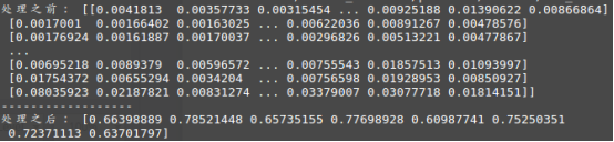
 可以看到，处理之前的数据明显比处理之后的数据多，而且处理之后的数据都是大于0.6的，说明generateBoundingBox函数对人脸框进行了一次初步的筛选。接着，我们对筛选后的人脸框显示到原图片上看看，添加如下代码，

# 显示人脸框
x1 = boxes[:, 0]
y1 = boxes[:, 1]
x2 = boxes[:, 2]
y2 = boxes[:, 3]
for i in range(len(boxes)):print(x1[i], y1[i], x2[i], y2[i])plt.gca().add_patch(plt.Rectangle((x1[i], y1[i]), x2[i] - x1[i], y2[i] - y1[i], edgecolor='w',facecolor='none'))# --韦访添加
plt.imshow(scale_img)
plt.show()
exit()

运行结果，

 哎，不对啊，没有哪个人脸框框对啊？此时你心里可能有一万匹草泥马在奔腾，别急，这只是检测了一个尺寸的框，我们将

# --韦访添加
plt.imshow(scale_img)
plt.show()
exit()

移到for循环外看看，运行结果，

 

这样是不是有很多框了？这也太多了吧？是的，P-Net初步检测到的框就是那么任性，所以才需要再经过nms再次筛选，我们也把nms筛选后的效果显示出来，

将

x1 = boxes[:, 0]
y1 = boxes[:, 1]
x2 = boxes[:, 2]
y2 = boxes[:, 3]
for i in range(len(boxes)):print(x1[i], y1[i], x2[i], y2[i])plt.gca().add_patch(plt.Rectangle((x1[i], y1[i]), x2[i] - x1[i], y2[i] - y1[i], edgecolor='w', facecolor='none'))

放到

if boxes.size>0 and pick.size>0:boxes = boxes[pick,:]total_boxes = np.append(total_boxes, boxes, axis=0)

里，运行效果如下，

是不是框少了很多啊？完整代码如下，

#将图片显示出来
# --韦访添加
plt.figure()
scale_img = img.copy()# first stage
#第一步，首先将图像缩放到不同尺寸形成“图像金字塔”
#然后，经过P-Net网络
for scale in scales:#宽高要取整hs=int(np.ceil(h*scale))ws=int(np.ceil(w*scale))#使用opencv的方法对图片进行缩放im_data = imresample(img, (hs, ws))#可视化的显示“图像金字塔”的效果# --韦访添加# scale_img[0:im_data.shape[0], 0:im_data.shape[1]] = 0# scale_img[0:im_data.shape[0], 0:im_data.shape[1]] = im_data[0:im_data.shape[0], 0:im_data.shape[1]]#对图片数据进行归一化处理im_data = (im_data-127.5)*0.0078125#增加一个维度，即batch size，因为我们这里每次只处理一张图片，其实batch size就是1img_x = np.expand_dims(im_data, 0)img_y = np.transpose(img_x, (0,2,1,3))# 送进P-Net网络# 假设img_y.shape=(1, 150, 150, 3)# 因为P-Net网络要经过3层核为3*3步长为1*1的卷积层，一层步长为2*2池化层# 所以conv4-2层输出形状为(1, 70, 70, 4)# 70是这么来的，(150-3+1)/1=148，经过池化层后为148/2=74，# 再经过一个卷积层(74-3+1)/1=72，再经过一个卷积层(72-3+1)/1=70# 计算方法参考博客：https://blog.csdn.net/rookie_wei/article/details/80146620# prob1层的输出形状为(1, 70, 70, 2)out = pnet(img_y)# 又变回来# out0的形状是(1, 70, 70, 4)# 返回的是可能是人脸的框的坐标out0 = np.transpose(out[0], (0,2,1,3))# out1的形状是(1, 70, 70, 2)# 返回的是对应与out0框中是人脸的可信度，第2个值为是人脸的概率out1 = np.transpose(out[1], (0,2,1,3))#out1[0,:,:,1]：表示框的可信度，只要一个值即可，因为这两个值相加严格等于1，这里只要获取“是”人脸框的概率#out0[0,:,:,:]：人脸框#scales:图片缩减比例#threshold:阈值，这里取0.6
#boxes返回值中，前4个值是还原比例后的人脸框坐标，第5个值是该人脸框中是人脸的概率，后4个值的未还原的人脸框坐标boxes, _ = generateBoundingBox(out1[0,:,:,1].copy(), out0[0,:,:,:].copy(), scale, threshold[0])#人脸框坐标对应的可信度# print('处理之前：', out1[0, :, :, 1])# print('------------------')# s = boxes[:, 4]# print('处理之后：', s)## # 显示人脸框# x1 = boxes[:, 0]# y1 = boxes[:, 1]# x2 = boxes[:, 2]# y2 = boxes[:, 3]# for i in range(len(boxes)):#     print(x1[i], y1[i], x2[i], y2[i])#     plt.gca().add_patch(plt.Rectangle((x1[i], y1[i]), x2[i] - x1[i], y2[i] - y1[i], edgecolor='w',facecolor='none'))# # --韦访添加# plt.imshow(scale_img)# plt.show()# exit()# inter-scale nms# 非极大值抑制，去掉重复的检测框pick = nms(boxes.copy(), 0.5, 'Union')if boxes.size>0 and pick.size>0:boxes = boxes[pick,:]total_boxes = np.append(total_boxes, boxes, axis=0)x1 = boxes[:, 0]y1 = boxes[:, 1]x2 = boxes[:, 2]y2 = boxes[:, 3]for i in range(len(boxes)):print(x1[i], y1[i], x2[i], y2[i])plt.gca().add_patch(plt.Rectangle((x1[i], y1[i]), x2[i] - x1[i], y2[i] - y1[i], edgecolor='w', facecolor='none'))# --韦访添加
plt.imshow(scale_img)
plt.show()
exit()

7、R-Net

继续往下看，

numbox = total_boxes.shape[0]
if numbox>0:# 再经过nms筛选掉一些可靠度更低的人脸框pick = nms(total_boxes.copy(), 0.7, 'Union')total_boxes = total_boxes[pick,:]#获取每个人脸框的宽高regw = total_boxes[:,2]-total_boxes[:,0]regh = total_boxes[:,3]-total_boxes[:,1]# 对人脸框坐标做一些处理，使得人脸框更紧凑qq1 = total_boxes[:,0]+total_boxes[:,5]*regwqq2 = total_boxes[:,1]+total_boxes[:,6]*reghqq3 = total_boxes[:,2]+total_boxes[:,7]*regwqq4 = total_boxes[:,3]+total_boxes[:,8]*reghtotal_boxes = np.transpose(np.vstack([qq1, qq2, qq3, qq4, total_boxes[:,4]]))total_boxes = rerec(total_boxes.copy())total_boxes[:,0:4] = np.fix(total_boxes[:,0:4]).astype(np.int32)dy, edy, dx, edx, y, ey, x, ex, tmpw, tmph = pad(total_boxes.copy(), w, h)

上面又对人脸框做一些微调，我们也可以可视化的看看，代码如下，

numbox = total_boxes.shape[0]
if numbox>0:# 再经过nms筛选掉一些可靠度更低的人脸框pick = nms(total_boxes.copy(), 0.7, 'Union')total_boxes = total_boxes[pick,:]#获取每个人脸框的宽高regw = total_boxes[:,2]-total_boxes[:,0]regh = total_boxes[:,3]-total_boxes[:,1]x1 = total_boxes[:, 0]y1 = total_boxes[:, 1]x2 = total_boxes[:, 2]y2 = total_boxes[:, 3]for i in range(len(total_boxes)):print(x1[i], y1[i], x2[i], y2[i])plt.gca().add_patch(plt.Rectangle((x1[i], y1[i]), x2[i] - x1[i], y2[i] - y1[i], edgecolor='w', facecolor='none'))# 对人脸框坐标做一些处理，使得人脸框更紧凑qq1 = total_boxes[:,0]+total_boxes[:,5]*regwqq2 = total_boxes[:,1]+total_boxes[:,6]*reghqq3 = total_boxes[:,2]+total_boxes[:,7]*regwqq4 = total_boxes[:,3]+total_boxes[:,8]*reghx1 = qq1y1 = qq2x2 = qq3y2 = qq4for i in range(len(total_boxes)):print('lll', x1[i], y1[i], x2[i], y2[i])plt.gca().add_patch(plt.Rectangle((x1[i], y1[i]), x2[i] - x1[i], y2[i] - y1[i], edgecolor='r', facecolor='none'))# --韦访添加plt.imshow(scale_img)plt.show()exit()total_boxes = np.transpose(np.vstack([qq1, qq2, qq3, qq4, total_boxes[:,4]]))total_boxes = rerec(total_boxes.copy())total_boxes[:,0:4] = np.fix(total_boxes[:,0:4]).astype(np.int32)dy, edy, dx, edx, y, ey, x, ex, tmpw, tmph = pad(total_boxes.copy(), w, h)

运行结果，

如上图所示，白框是调整之前的，框比较大，红色的是调整后的，显得更“紧凑”些。

继续往下看，就是R-Net了，代码如下，

#第二步，经过R-Net网络
numbox = total_boxes.shape[0]
if numbox>0:# second stagetempimg = np.zeros((24,24,3,numbox))for k in range(0,numbox):tmp = np.zeros((int(tmph[k]),int(tmpw[k]),3))tmp[dy[k]-1:edy[k],dx[k]-1:edx[k],:] = img[y[k]-1:ey[k],x[k]-1:ex[k],:]if tmp.shape[0]>0 and tmp.shape[1]>0 or tmp.shape[0]==0 and tmp.shape[1]==0:#R-Net输入大小为24*24，所以要进行缩放tempimg[:,:,:,k] = imresample(tmp, (24, 24))else:return np.empty()tempimg = (tempimg-127.5)*0.0078125tempimg1 = np.transpose(tempimg, (3,1,0,2))#经过R-Net网络out = rnet(tempimg1)out0 = np.transpose(out[0])out1 = np.transpose(out[1])score = out1[1,:]ipass = np.where(score>threshold[1])total_boxes = np.hstack([total_boxes[ipass[0],0:4].copy(), np.expand_dims(score[ipass].copy(),1)])mv = out0[:,ipass[0]]if total_boxes.shape[0]>0:pick = nms(total_boxes, 0.7, 'Union')total_boxes = total_boxes[pick,:]total_boxes = bbreg(total_boxes.copy(), np.transpose(mv[:,pick]))total_boxes = rerec(total_boxes.copy())

就不一一分析了。

8、O-Net

接着就是O-Net网络了，代码如下，

#第三步，经过O-Net网络
numbox = total_boxes.shape[0]
if numbox>0:# third stagetotal_boxes = np.fix(total_boxes).astype(np.int32)dy, edy, dx, edx, y, ey, x, ex, tmpw, tmph = pad(total_boxes.copy(), w, h)tempimg = np.zeros((48,48,3,numbox))for k in range(0,numbox):tmp = np.zeros((int(tmph[k]),int(tmpw[k]),3))tmp[dy[k]-1:edy[k],dx[k]-1:edx[k],:] = img[y[k]-1:ey[k],x[k]-1:ex[k],:]if tmp.shape[0]>0 and tmp.shape[1]>0 or tmp.shape[0]==0 and tmp.shape[1]==0:# O-Net输入大小为48*48，所以要进行缩放tempimg[:,:,:,k] = imresample(tmp, (48, 48))else:return np.empty()tempimg = (tempimg-127.5)*0.0078125tempimg1 = np.transpose(tempimg, (3,1,0,2))# 经过O-Net网络out = onet(tempimg1)out0 = np.transpose(out[0])out1 = np.transpose(out[1])out2 = np.transpose(out[2])score = out2[1,:]points = out1ipass = np.where(score>threshold[2])points = points[:,ipass[0]]total_boxes = np.hstack([total_boxes[ipass[0],0:4].copy(), np.expand_dims(score[ipass].copy(),1)])mv = out0[:,ipass[0]]w = total_boxes[:,2]-total_boxes[:,0]+1h = total_boxes[:,3]-total_boxes[:,1]+1points[0:5,:] = np.tile(w,(5, 1))*points[0:5,:] + np.tile(total_boxes[:,0],(5, 1))-1points[5:10,:] = np.tile(h,(5, 1))*points[5:10,:] + np.tile(total_boxes[:,1],(5, 1))-1if total_boxes.shape[0]>0:total_boxes = bbreg(total_boxes.copy(), np.transpose(mv))pick = nms(total_boxes.copy(), 0.7, 'Min')total_boxes = total_boxes[pick,:]points = points[:,pick]

其中，total_boxes包含的就是我们需要的人脸框数据，points就是五个关键点坐标，

#显示人脸框和关键点
for i in range(len(total_boxes)):x1 = total_boxes[:, 0]y1 = total_boxes[:, 1]x2 = total_boxes[:, 2]y2 = total_boxes[:, 3]print('lll', x1[i], y1[i], x2[i], y2[i])plt.gca().add_patch(plt.Rectangle((x1[i], y1[i]), x2[i] - x1[i], y2[i] - y1[i], edgecolor='r', facecolor='none'))plt.scatter(points[0], points[5], c='red')
plt.scatter(points[1], points[6], c='red')
plt.scatter(points[2], points[7], c='red')
plt.scatter(points[3], points[8], c='red')
plt.scatter(points[4], points[9], c='red')plt.imshow(scale_img)
plt.show()
exit()

运行结果，

自此，我们的分析就完成了。得出人脸框和关键点后，就可以根据眼睛的关键点将眼睛“扣”出来（有点血腥哈），再送给上一讲的开闭眼识别，就可以知道是否在闭眼了。识别是否打哈欠，是否也可以根据嘴巴的关键点将嘴巴扣出来，然后再训练一个神经网络来识别是否在打哈欠？当然，这个还得考虑到嘴巴张开的程度和时间等等因素。为了方便看注释，我将注释后的代码上传了，链接如下，如有分析错误的，请指教。

https://download.csdn.net/download/rookie_wei/10938739

 

-------------------------------------------------------------------------------------

20190602补充

结合opencv实时的将眼睛框出来的博客链接如下，

https://blog.csdn.net/rookie_wei/article/details/90744341

 

如果您感觉本篇博客对您有帮助，请打开支付宝，领个红包支持一下，祝您扫到99元，谢谢～～

 

这篇关于tensorflow入门教程(三十五)facenet源码分析之MTCNN--人脸检测及关键点检测的文章就介绍到这儿，希望我们推荐的文章对编程师们有所帮助！

---