深度学习-从零开始(2) - LinearRegression

本文主要是介绍深度学习-从零开始(2) - LinearRegression，希望对大家解决编程问题提供一定的参考价值，需要的开发者们随着小编来一起学习吧！

本章背景

本章是来源于coursera课程 python-machine-learning中的作业2内容。

本章内容

多项式线性回归
决定系数 R2 (coefficient of determination) 的计算
ridge线性回归
lasso线性回归

参考

评价回归模型
r2_score为负数的问题探讨

0. Polynomial LinearRegression(多项式线性回归)

随机创建如下数据：

import numpy as np
import pandas as pd
from sklearn.model_selection import train_test_splitnp.random.seed(0)
n = 15
x = np.linspace(0,10,n) + np.random.randn(n)/5
y = np.sin(x)+x/6 + np.random.randn(n)/10X_train, X_test, y_train, y_test = train_test_split(x, y, random_state=0)

创建特定维度的多项式线性回归：

使用degree = 1,3,6 and 9 来训练X_train，并随机生成一些预测数据验证拟合结果：

def test_1():from sklearn.linear_model import LinearRegressionfrom sklearn.preprocessing import PolynomialFeaturesxx_pred = np.linspace(0, 10, 100)degrees = [1, 3, 6, 9]results = []for index in range(0, 4):degree = degrees[index]regression = LinearRegression()featurizer = PolynomialFeatures(degree=degree)X_train_features = featurizer.fit_transform(X_train.reshape(-1, 1))regression.fit(X_train_features, y_train.reshape(-1, 1))xx_pred_features = featurizer.transform(xx_pred.reshape(-1, 1))yy_pred = regression.predict(xx_pred_features)# append the resultsresults.append(yy_pred.reshape(1, -1))return np.concatenate(results)# 将几个维度的多项式拟合曲线绘制出来
def plot_results(degree_predictions):import matplotlib.pyplot as pltplt.figure(figsize=(10,5))plt.plot(X_train, y_train, 'o', label='training data', markersize=10)plt.plot(X_test, y_test, 'o', label='test data', markersize=10)for i,degree in enumerate([1,3,6,9]):plt.plot(np.linspace(0,10,100), degree_predictions[i], alpha=0.8, lw=2, label='degree={}'.format(degree))plt.ylim(-1,2.5)plt.legend(loc=4)plt.show()plot_results(test_1())

1. coefficient of determination (决定系数R2)

决定系数(coefficient of determination)的计算方法：
R2-score公式
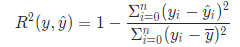
R^{2期待值越接近1说明拟合越好，越接近0说明拟合结果差。同时根据公式可以发现，在实际计算中R}2是可能为负数的，通过简单计算，当R^2为负数时,说明:
当R2-score为负数
说明拟合结果差到不如使用均值。
还是使用上面的数据，分别计算X_train 和 X_test的R^2:

def test_2():from sklearn.linear_model import LinearRegressionfrom sklearn.preprocessing import PolynomialFeaturesfrom sklearn.metrics.regression import r2_score# Your code hereresults = []model_cnt = 10result_train = []result_test = []for degree in range(0, model_cnt):linearRegression = LinearRegression()featurizer = PolynomialFeatures(degree=degree)X_train_features = featurizer.fit_transform(X_train.reshape(-1, 1))y_train_features = y_train.reshape(-1, 1)linearRegression.fit(X_train_features, y_train_features)y_train_pred = linearRegression.predict(X_train_features)print('X_train r2_score ==> : ', r2_score(y_train_features, y_train_pred))result_train.append(r2_score(y_train_features, y_train_pred))# calculate the values for Test setX_test_features = featurizer.transform(X_test.reshape(-1, 1))y_test_pred = linearRegression.predict(X_test_features)y_test_features = y_test.reshape(-1, 1)print('X_test r2-score ==> : ', r2_score(y_test_features, y_test_pred))result_test.append(r2_score(y_test_features, y_test_pred))results.append(np.array(result_train).reshape(10, ))results.append(np.array(result_test).reshape(10, ))print(results[0].shape, results[1].shape)print(results)return results# Your answer here

从代码中也可以看出来，在sklearn工具包中已经包含了r2_score的计算函数，直接传入真实值和预测值即可计算，当然可以通过如上公式自行计算。

2. Ridge线性回归

Ridge线性回归是改良后的最小二乘法, 是有偏估计的回归方法, 即给损失函数加上一个正则化项, 也叫惩罚项(L2范数),防止过拟合。

Ridge回归的特点是以损失部分信息、降低精度为代价获得回归系数更为符合实际、更可靠的回归方法，对病态数据的拟合要强于最小二乘法。

Ridge的公式如下
Ridge回归损失函数
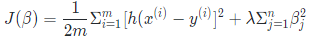
其中, m是样本量, n是特征数, λ是惩罚项参数(其取值大于0), 加惩罚项主要为了让模型参数的取值不能过大. 当λ趋于无穷大时, 对应βj趋向于0, 而βj表示的是因变量随着某一自变量改变一个单位而变化的数值(假设其他自变量均保持不变), 这时, 自变量之间的共线性对因变量的影响几乎不存在, 故其能有效解决自变量之间的多重共线性问题, 同时也能防止过拟合.

代码示例：

    import numpy as npimport pandas as pdfrom sklearn.model_selection import train_test_splitfrom matplotlib.pyplot import MultipleLocatorfrom sklearn.preprocessing import PolynomialFeaturesfrom sklearn.linear_model import Lasso, LinearRegression, Ridgefrom sklearn.metrics.regression import r2_scorenp.random.seed(0)n = 15x = np.linspace(0, 10, n) + np.random.randn(n) / 5y = np.sin(x) + x / 6 + np.random.randn(n) / 10X_train, X_test, y_train, y_test = train_test_split(x, y, random_state=0)# Your code herenormalLinearRegression = LinearRegression()ridgeLinearRegression = Ridge(alpha=0.01, max_iter=10000, solver='svd')featurizer = PolynomialFeatures(degree=12)X_train_features = featurizer.fit_transform(X_train.reshape(-1, 1))X_test_features = featurizer.transform(X_test.reshape(-1, 1))# train the non-regularized linearRegression modelnormalLinearRegression.fit(X_train_features, y_train.reshape(-1, 1))y_test_pred_normal = normalLinearRegression.predict(X_test_features)# cal the R2 score for non-regularized modelr2_score_normal = r2_score(y_test.reshape(-1, 1), y_test_pred_normal)print('non-regularized linearRegression r2-score ==> ', r2_score_normal)# train the ridge linearRegression modelridgeLinearRegression.fit(X_train_features, y_train.reshape(-1, 1))y_test_pred_ridge = ridgeLinearRegression.predict(X_test_features)# cal the R2-score for Ridge-regressionr2_score_ridge = r2_score(y_test.reshape(-1, 1), y_test_pred_ridge)print('ridge-regularized linearRegression r2-score ==> ', r2_score_ridge)

Ridge回归并不能解决减少系数/维度数量的问题，其系数均不为0。

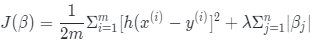
3. LASSO线性回归

模型参数越多复杂度越高，即使用线性回归依然有很多的参数需要训练，并且这也会造成一定程度上的过拟合。并且最终得到的模型的可解释性也不高。这个时候可以考虑引入lasso回归。

Lasso回归的特点是可以在拟合训练数据的同时进行变量选择（Variable Selection）。那么它是通过什么机制选择的呢？答案就是：正则化（Regularization）！或者可以简单的把这个东西叫做惩罚项。

LASSO的公式如下
Lasso回归损失函数
代码示例：

    import numpy as npimport pandas as pdfrom sklearn.model_selection import train_test_splitfrom matplotlib.pyplot import MultipleLocatorfrom sklearn.preprocessing import PolynomialFeaturesfrom sklearn.linear_model import Lasso, LinearRegression, Ridgefrom sklearn.metrics.regression import r2_scorenp.random.seed(0)n = 15x = np.linspace(0, 10, n) + np.random.randn(n) / 5y = np.sin(x) + x / 6 + np.random.randn(n) / 10X_train, X_test, y_train, y_test = train_test_split(x, y, random_state=0)# Your code herenormalLinearRegression = LinearRegression()ridgeLinearRegression = Ridge(alpha=0.01, max_iter=10000, solver='svd')featurizer = PolynomialFeatures(degree=12)X_train_features = featurizer.fit_transform(X_train.reshape(-1, 1))X_test_features = featurizer.transform(X_test.reshape(-1, 1))# train the non-regularized linearRegression modelnormalLinearRegression.fit(X_train_features, y_train.reshape(-1, 1))y_test_pred_normal = normalLinearRegression.predict(X_test_features)# cal the R2 score for non-regularized modelr2_score_normal = r2_score(y_test.reshape(-1, 1), y_test_pred_normal)print('non-regularized linearRegression r2-score ==> ', r2_score_normal)# train the lasso linearRegression modellassoLinearRegression.fit(X_train_features, y_train.reshape(-1, 1))y_test_pred_lasso = lassoLinearRegression.predict(X_test_features)# cal the R2 score for lasso-regularized modelr2_score_lasso = r2_score(y_test.reshape(-1, 1), y_test_pred_lasso)print('lasso-regularized linearRegression r2-score ==> ', r2_score_lasso)

Lasso回归可以解决减少系数/维度数量的问题，其部分系数为0。

这篇关于深度学习-从零开始(2) - LinearRegression的文章就介绍到这儿，希望我们推荐的文章对编程师们有所帮助！