本文主要是介绍深度学习入门(上)01(用cifar数据实现三层网络实现图片分类),希望对大家解决编程问题提供一定的参考价值,需要的开发者们随着小编来一起学习吧!
目录
1-1深度学习入门-imagenet图像分类比赛
1-2计算机视觉面临的挑战和常规套路
1-3 K近邻进行图像分类
KNN的实现步骤
KNN总结
KNN的问题:
数据库样例:
测试结果
最近邻实现代码
1-4 超参数与交叉验证
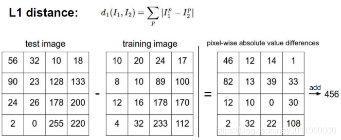
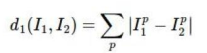
L1 manhanttan距离
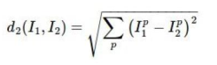
L2 euclidean欧式距离
超参数的问题:
找到最好的参数
测试结果
结论:K近邻用于图像计算不可取
KNN方法用于图像识别总结
KNN方法用于图像识别步骤
1-5 线性分类
1-6 损失函数
1-7正则化惩罚项
对比W1和W2两种权重模型的效果
1-8 softmax分类器
svm和softmax两种损失函数对比
1-9最优化形象解读
1-10 梯度下降算法原理
1-11 反向传播
2-1神经网络整体架构
神经网络结构:
激活函数
2-2神经网络模型实例演示
2-3 过拟合问题解决方案
神经网络整体流程;
数据预处理
权重初始化
DROP-OUT
3-1python环境搭建
3-2 eclipse 搭建python环境,选择IDE
3-3 深度学习入门
3-5 神经网络案例-cifar分类任务
cifar数据集
3-6 神经网络案例-分模块构造神经网络
3-7 神经网络案例-训练神经网络完成
cifar-10 dataset
数据集http://www.cs.toronto.edu/~kriz/cifar.html
1-1深度学习入门-imagenet图像分类比赛
官网http://www.image-net.org/
数据集介绍https://blog.csdn.net/fengbingchun/article/details/88606621
2012年alexnet卷积神经网络

百度人工智能实验室
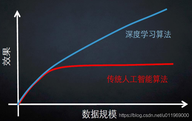
深度学习使用的神经网络是机器学习算法的分支
1-2计算机视觉面临的挑战和常规套路
图像分类
一张图片被表示成三维数组的形式,每个像素的值从0到255(像素点越大亮度越高),300*100*3:长宽颜色通道EGB
图像识别的挑战:照射角度,光照强度,形状改变,部分遮蔽,背景混入

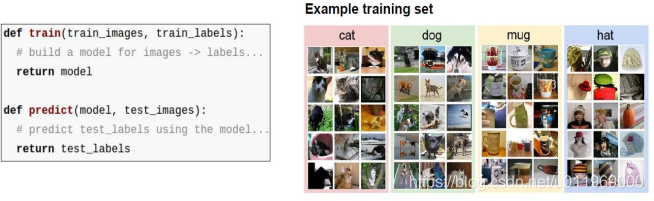
常规套路
1、收集数据并给定标签
2、训练一个分类器
3、测试,评估
1-3 K近邻进行图像分类
Knn原理
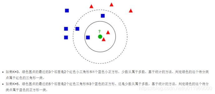
KNN的实现步骤
对于未知类别属性数据集中的点,
1、计算已知类别数据集中的点与当前点的距离
2、按照距离一次排序
3、选取与当前距离最小的K个点
4、确定前K个点所在的类别的出现概率
5、返回前K个点出现频率最高的类别作为当前点预测分类
KNN总结
knn算法本身简单有效,是一种lazy-learning算法
分类器不需要训练数据集,训练时间复杂度为0,
knn分类的计算复杂度和训练集中的文档数目成正比,训练集中文档总数为n,那么KNN的分类时间复杂度为o(n)
KNN三要素:k值选择,距离度量和分类决策规则
KNN的问题:
该算法在分类时有个主要的不足是,当样本不平衡时,如一个类的样本容量很大,而其他类样本容量很
小时,有可能导致当输入一个新样本时,该样本的 K 个邻居中大容量类的样本占多数
解决:不同的样本给予不同权重项
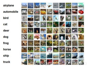
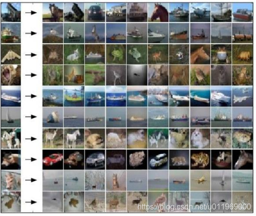
数据库样例:
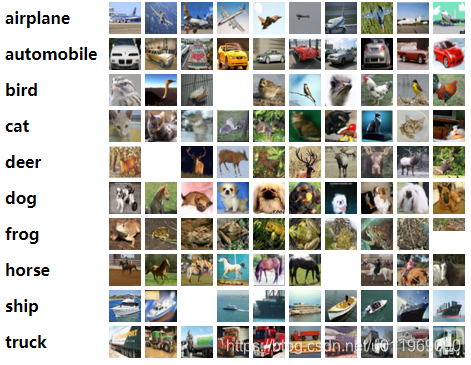
CIFAR-10
10类标签,(airplane,automobile,bird,cat,deer,dog,frog,hurse,ship,truck)
50000个训练数据,10000个测试数据,大小均为32*32
如何计算:
用k近邻来进行图像分类,即为对图像像素点的计算,
测试结果
最近邻实现代码
import numpy as np
#KNN实现代码
class NearestNeighbor:def __init__(self):passdef train(self, X, y):#记录所有的训练数据,X=N*D Y=种类数self.Xtr = Xself.ytr = ydef predict(self, X):num_test = X.shape[0]Ypred = np.zeros(num_test, dtype= self.ytr.dtype)#对于每一个测试数据找到与其l1举例最小的样本的标签作为它的标签for i in range(num_test):distances = np.sum(np.abs(self.Xtr - X[i, :]),axis = 1)min_index = np.argmin(distances)Ypred[i] = self.ytr[min_index]return Ypred
1-4 超参数与交叉验证
超参数,就是在训练中可以改变的参数,比如knn中的距离计算公式
L1 manhanttan距离
L2 euclidean欧式距离
超参数的问题:
1、距离如何设定
2、knn中的k如何设定
3、其他超参数如何设定
找到最好的参数
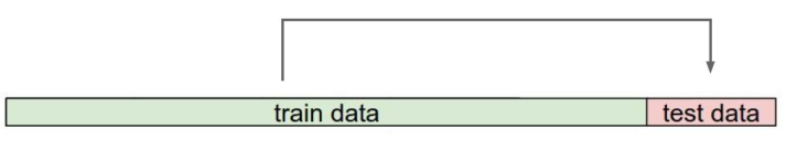
Train_data 70%,test_data 30%
多次用测试数据试验,找到做好的一组参数组合?
错误的的想法,测试数据只能最终用
测试集只能在最终使用
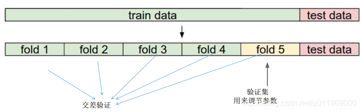
交叉验证70%的train_data里面切割为n个fold,其中一个为验证集
1,2,3,4→5
5,2,3,4→1
1,5,3,4→2
1,2,5,4→3
1,2,3,5→4
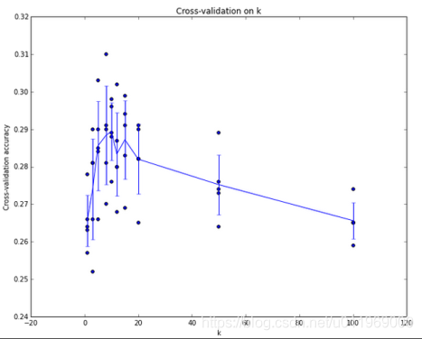
测试结果
x轴为k的大小,y轴为交叉验证准确率
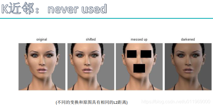
结论:K近邻用于图像计算不可取
1、背景主导:knn在计算距离的时候,由于图中识别的物体只占少部分,把背景考虑进来了
2、不同的变换(偏离,遮挡,灰度)和原图具有相同的L2距离
KNN方法用于图像识别总结
1.选取超参数的正确方法是:将原始训练集分为训练集和验证集,我们在验证集上尝试不同的超参数,最后保留表现最好那个
2.如果训练数据量不够,使用交叉验证方法,它能帮助我们在选取最优超参数的时候减少噪音。
3.一旦找到最优的超参数,就让算法以该参数在测试集跑且只跑一次,并根据测试结果评价算法。
4.最近邻分类器能够在CIFAR-10上得到将近40%的准确率。该算法简单易实现,但需要存储所有训练数据,并且在测试的时候过于耗费计算能力
5.最后,我们知道了仅仅使用L1和L2范数来进行像素比较是不够的,图像更多的是按照背景和颜色被分类,而不是语义主体分身
KNN方法用于图像识别步骤
1.预处理你的数据:对你数据中的特征进行归一化(normalize),让其具有零平均值(zero mean)和单位方差(unit variance) 。
2.如果数据是高维数据,考虑使用降维方法,比如PCA
3.将数据随机分入训练集和验证集。按照一般规律, 70%-90% 数据作为训练集
4.在验证集上调优,尝试足够多的k值,尝试L1和L2两种范数计算方式。
发现不同的变换和原图具有相同的L2距离故K近邻不能用于图像识别
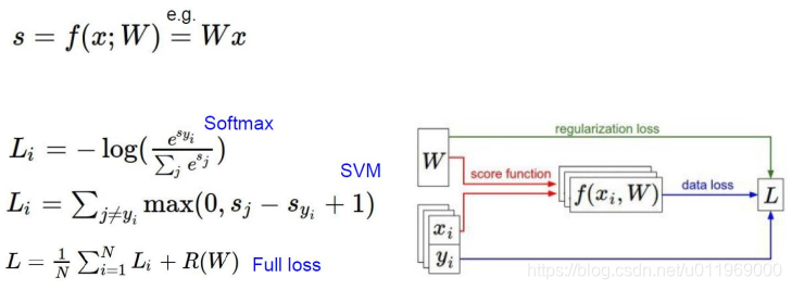
1-5 线性分类
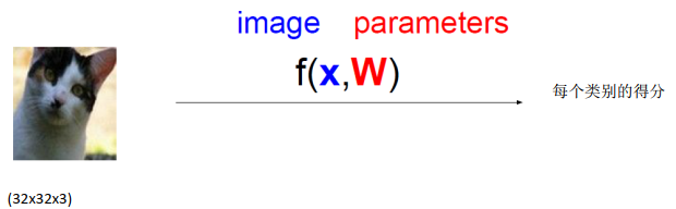
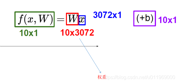
输入x:32*32*3个像素点,W权重矩阵,b截距
输出b:10个类别的得分概率
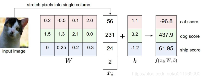
得分值高位最终的结果值
线性分类,是按线性划分区域
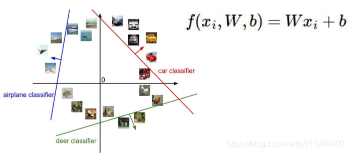
出现预测错了,则需要改正
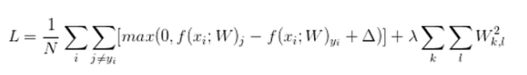
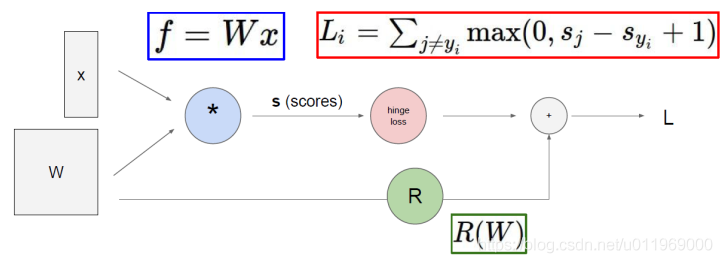
1-6 损失函数
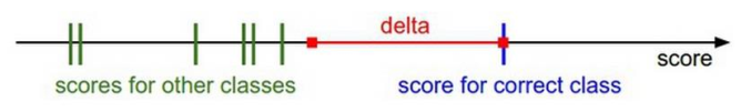
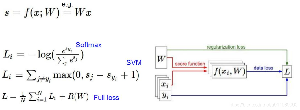
SVM损失函数
Sj是其他J个类别的概率,Syi准确的类别的概率
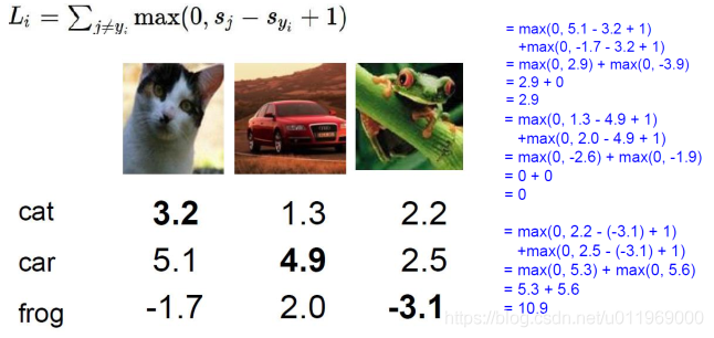
+1(delta):可容忍程度,偏离的大小小于1则不计
<0的损失不计入。>0计入算是
1-7正则化惩罚项
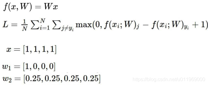
对比W1和W2两种权重模型的效果
W1的权重至考虑x1这个像素点,其他3个像素点可以为任何职,W2在像素点的权重比较均匀,惩罚项小
为了选到W2这样的权重,原始损失函数需加上正则化惩罚项,惩罚项惩罚权重参数
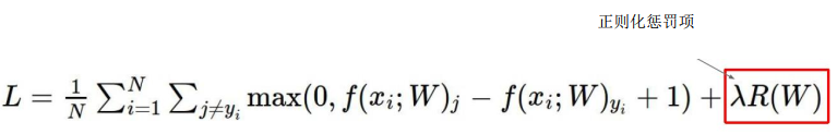
R(W)用来l2正则化
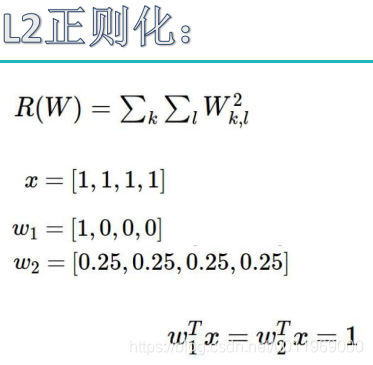
L1=1>L2=1/4,L1惩罚得比较多
SVM损失函数终极版
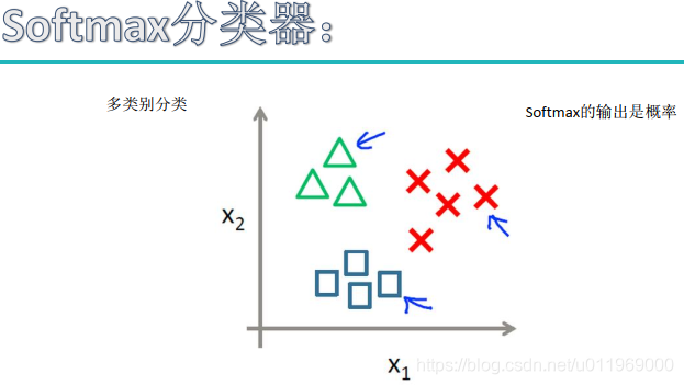
1-8 softmax分类器

sigmoid把任意实数变成0-1的概率值
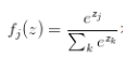
softmax函数
softmax分类器的作用
softmax的输出,是归一化的分类概率
损失函数(交叉熵损失,cross-entropy loss)
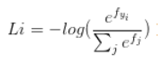
输入:一个向量,向量中元素为任意实数的评分值
输出:一个向量,每个元素值在0-1之间,且所有元素之和为1
示例:
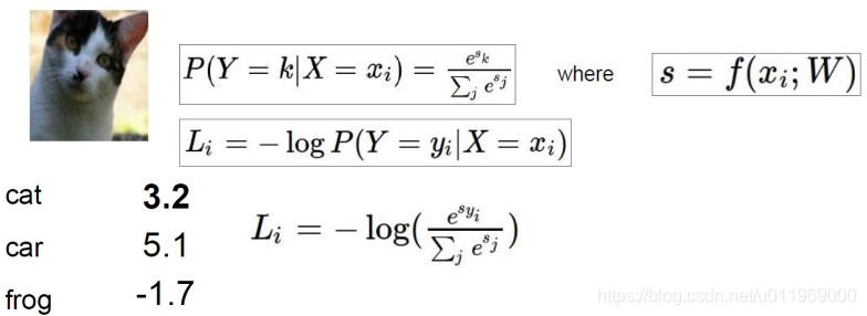
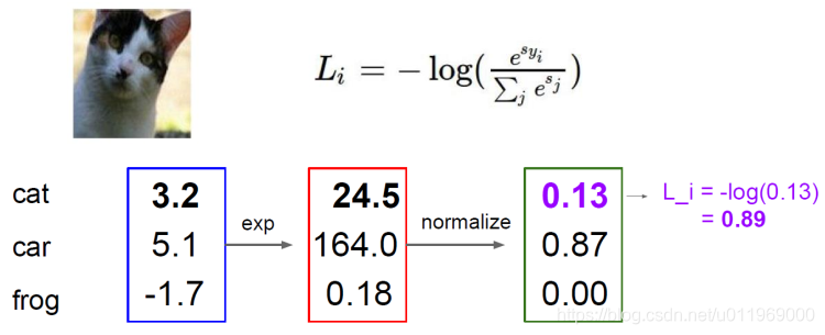
eg:exp(3.2) ,归一化,-log(),
e的x次幂,如果是负数为变成很小的值,
归一化操作,概率值且和为1
拿cat的正确类别的损失值Li
svm和softmax两种损失函数对比
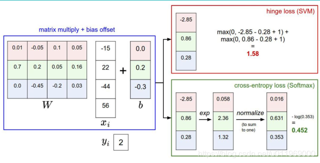
svm的损失函数,对错误类别的差异不大, 不用
一般用softmax函数计算损失函数
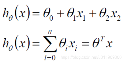
1-9最优化形象解读
一步步喂数据,一步步优化θ参数,迭代优化的过程很重要
h(x)为线性回归公式
y为第i个参数的预测模型
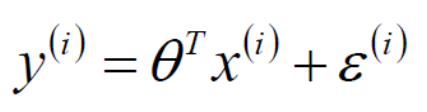
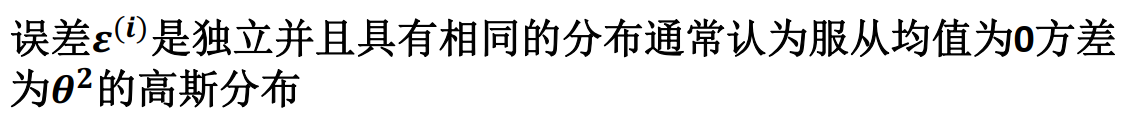
根据误差的正态分布特性
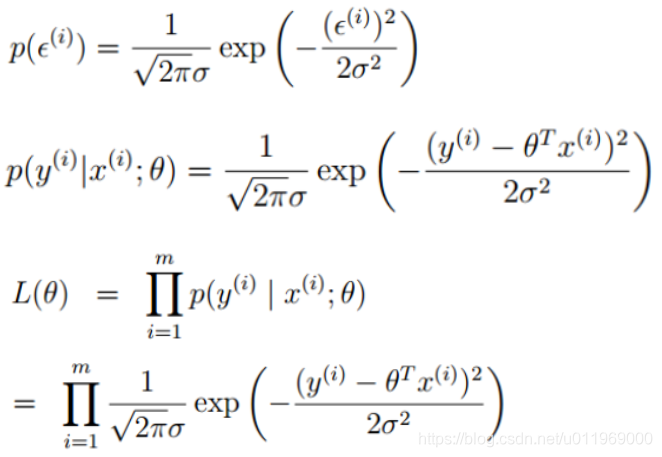
J(θ)为待优化的建模函数
粗暴的方法代码实现及结果:
import numpy as np
#粗暴的想法,直接到山底
#X_trian为传入数据矩阵,如3073*50000
#y_train为图片的类别标签概率值,如10*50000
#假设L函数来估计损失函数
bestloss = float("inf")
for num in range(1000):W = np.random.randn(10, 3073) * 0.0001loss = L(X_trian, Y_train, W)if loss < bestloss:bestloss = loss bestW = Wprint ('in attempt %d the loss was %f,best %f' %(num,loss,bestloss))
#粗暴想法的结果
#假设X_test是3073*10000,Y_test为10000*1
#scores为10*10000,每一类的分数矩阵
scores = Wbest.dot(Xte_cols)
#获取最高分的类别
Yte_prediect = np.argmax(scores ,axis = 0)
#计算平均预测准确精度
np.mean(Yte_predict == Yte)
m=10,沿着坡度下山最快,坡度为切线
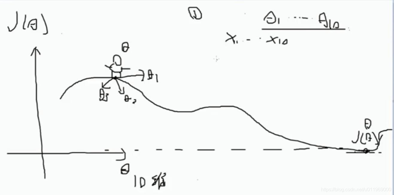
跟随梯度函数
Bachsize通常是2的整数倍(32, 64, 128)2的整数次幂
#找打山坡最低点
#生成随机初始权重W
W = np.random.randn(10,3073)*0.001
bestloss = float("inf")
for i in range(1000):step_size = 0.0001Wtry = W + np.random.randn(10,3073) * step_sizeloss = L(Xtr_cols,Ytr,Wtry)if loss < bestloss:W = Wtrybestloss = lossprint ('iter %d loss is %f') % (i ,bestloss)
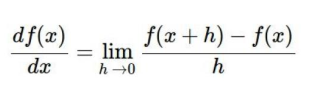
#跟随梯度
def eval_numerical_gradient(f,x):fx = f(x)grad = np.zeros(x.shape)h = 0.00001it = np.nditer(x,flags=['multi_index'],op_flags = ['readwrite'])while not it.finished:#f(x+h)ix = it.multi_indexold_value = x[ix]x[ix] = old_value + h #增加hfxh = f(x) #估计f(x+h)x[ix] = old_valuegrad[ix] = (fxh - fx) / hit.iternext()return grad
#梯度下降,bacthsize 通常是2的整数倍,32,64,128,256
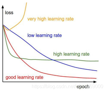
while True:data_batch = sample_training_data(data, 256)weight_grad = evaluate_gradient(loss_fun, data_batch, weights)weights += - step_size * weight_grad#学习步长*更新梯度训练网络时,loss值的可视化结果
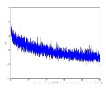
学习率:一次学习多大,△w多大,一般设置学习率设置为0.0001
通过小的学习率大的跌打次数进行训练
训练网络时的LOSS值视化结果
1-10 梯度下降算法原理
X 到loss 前向传播
BP算法是前向传播
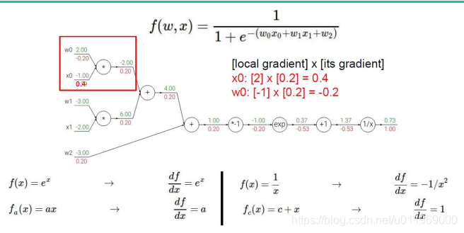
1-11 反向传播

最优化体现在反向传播
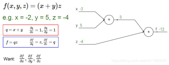
分别计算x,y,z对l的影响
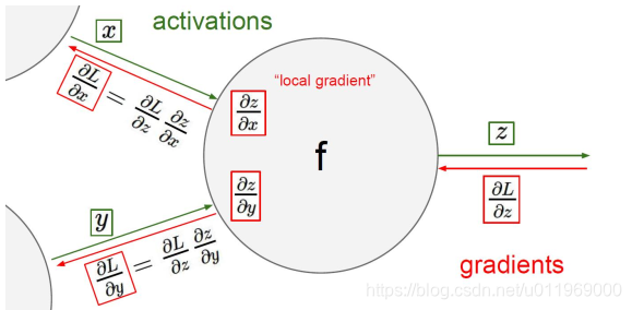
把公式量化,量式法则
sigmoid函数的一步一步求导向前传
整体求导,先求sigmoid函数再求线性回归,
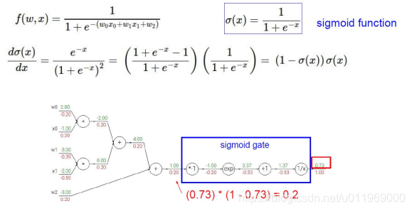
引入门单元
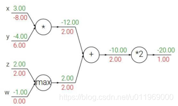
加法门单元:均等分配,求偏导都为1
MAX门单元:给最大的,把梯度分为较大的值,
乘法门单元:互换,q对x求偏导为y,对y求偏导为x梯度互换
2-1神经网络整体架构
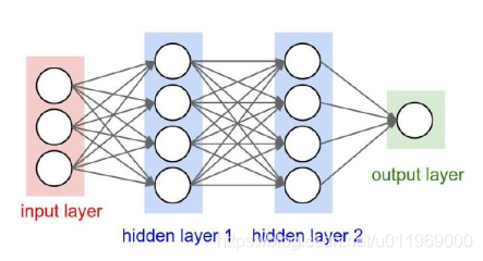
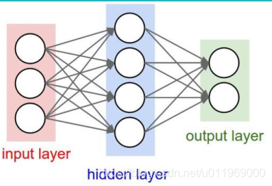
神经网络结构:
层次的结构(神经网络是由权重参数的组合构成):
输入层(x1,x2,x3),隐藏层1(W1),隐藏层2(W1)和输出层out
隐藏层:权重的中间计算结果,第一层的权重系数,第二层,第n层
比如(W3(W2(W1*X1)))=OUT
神经网络必须指定的参数:Wx
为啥存在多个隐藏层Wx:隐藏层中包含激活函数,如下非线性中的Max()可视为激活函数
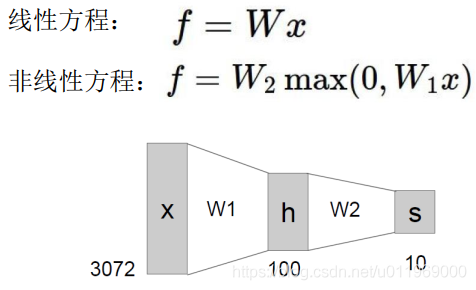
非线性方程中包含单层,多层

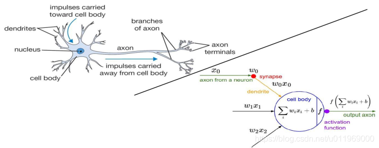
激活函数
因线性函数的分类能力不够,增加非线性函数加强模型能力,激活函数加强神经网络的效果
比如sigmoid函数吧线性压缩成非线性sigmoid(W1*x)
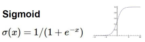
当取负无穷为0,正无穷为1,出现的问题:
正向传播,分步求导,每次梯度都要累乘,
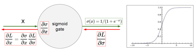
sigmoid的导数为切线, 当值越大或越小,越接近0,出现梯度消失,
sigmoid被淘汰,因梯度消失太严重
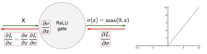
引入RELU函数作为激活函数
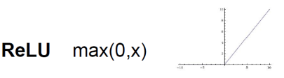
X<0都为0,求导简单
2-2神经网络模型实例演示
谷歌神经网络游乐园
http://playground.tensorflow.org/
斯坦福提供的一个用java-script写的2层隐藏层的训练网络
https://cs.stanford.edu/people/karpathy/convnetjs/demo/classify2d.html
layer_defs = [];
layer_defs.push({type:'input', out_sx:1, out_sy:1, out_depth:2});
layer_defs.push({type:'fc', num_neurons:10, activation: 'tanh'});#设置隐藏层1
layer_defs.push({type:'fc', num_neurons:10, activation: 'tanh'});#设置隐藏层2
layer_defs.push({type:'softmax', num_classes:2});
net = new convnetjs.Net();
net.makeLayers(layer_defs);
trainer = new convnetjs.SGDTrainer(net, {learning_rate:0.01, momentum:0.1, batch_size:10, l2_decay:0.001});
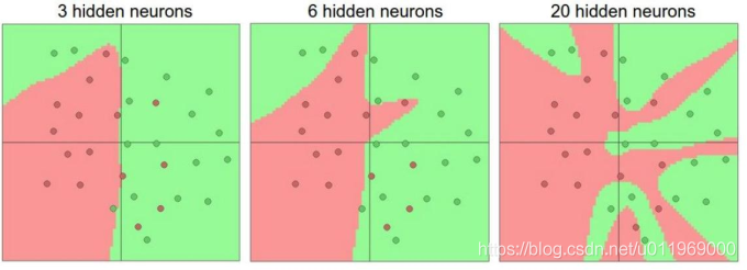
对于模型训练而言(比如环绕型数据),隐藏层设置越多,效果越好
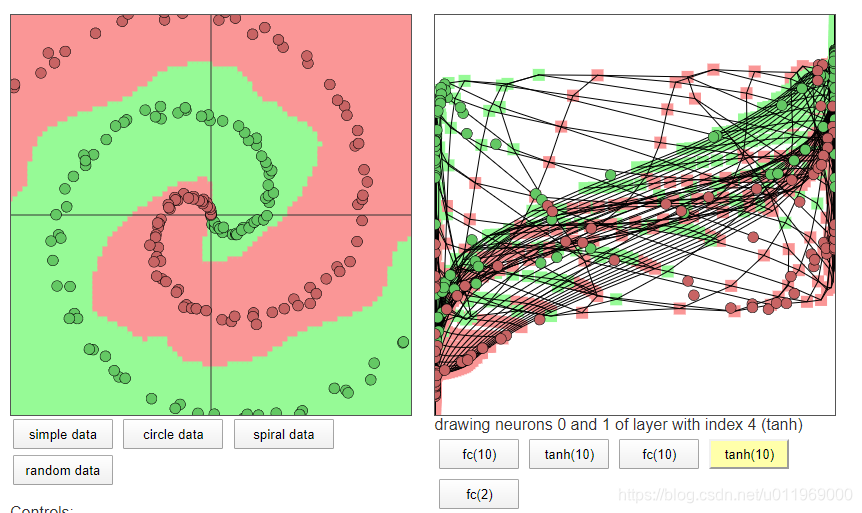
神经网络层越多,过拟合现象越明显
2-3 过拟合问题解决方案
神经网络的特点:W1,W2无法解释
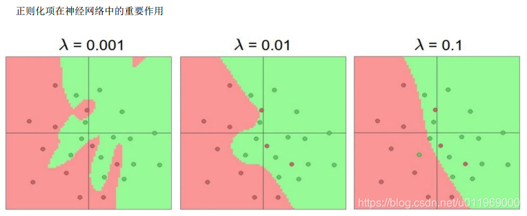
正则化的作用,λW^2
λ较小的时候,为了中间的红色,或拟合出一个圈,但实际测试数据分布来说,这个点为绿色的概率比较大,出现过拟合,部分错误点,异常点,离群点影响了结果
λ较大的时候,模型较平滑,泛化能力越强,
神经元越多,越能表达复杂的模型,但过拟合的危险越大
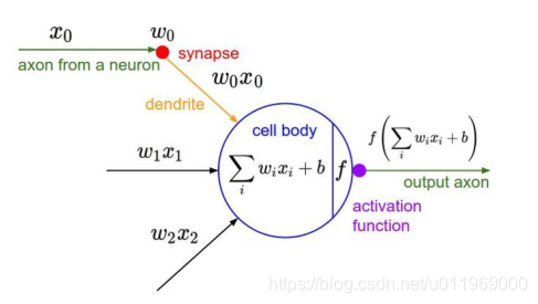
神经网络整体流程;
输入x0,x1,x2,经过w1,w2,w3组合之后,经过激活函数产生非线性模型效果
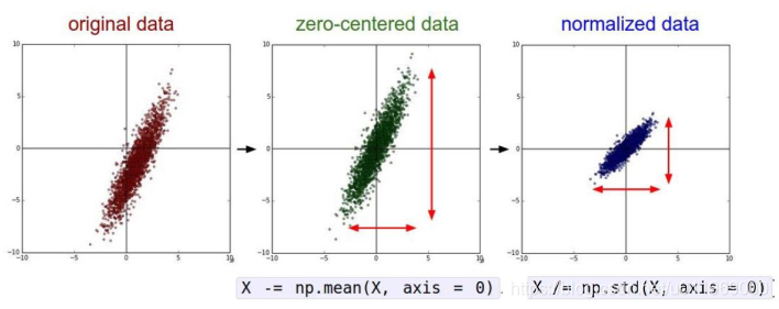
数据预处理
原始数据(0-255)→(均值为0)0为中心点数据→(除以标准差)归一化数据
权重初始化
初始值为0,训练不出来都是0
初始值方式:随机初始化,高斯初始化
随机初始化
W=0.0.1*np.random.randn(D,H)
对于b,0值或1值初始化。
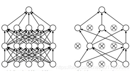
DROP-OUT
(左)全连接操作:每个神经元,每个x和w都连接,容易过拟合,
(右)drop-out:对于部分w1,w3,w4不用传播了,每次迭代,随机选择指定drop-out率为60%,只留下60%的神经元进行前向和反向传播,显得神经网络不那么臃肿,降低过拟合的风险,
目前的神经网络都会drop-out
3-1python环境搭建
1、下载python
2、配置系统环境变化
3、配置库
Numpy
用conda安装,或者pip安装
conda集成了python和python库
conda list
jupyter:可视化显示,debug麻烦
用ananconda查找适配的包机安装
ananconda search -t conda tensorflow
Ananconda show dhirschfeld/tensorflow
conda install --channel https://conda.anaconda.org/Paddle paddlepaddle-gpu
conda install --channel https://pypi.tuna.tsinghua.edu.cn/simple paddlepaddle-gpu
3-2 eclipse 搭建python环境,选择IDE
选择自己舒服的环境,
eclipse一般用来写java,需要在java的环境运行,需要配置jdk,
下载python编译插件
Name:PyDev
Location:网站
配置IDE环境中的python编译器环境
新增interpreter
本实验用vscode
3-3 深度学习入门
写一个只有三层的神经网络
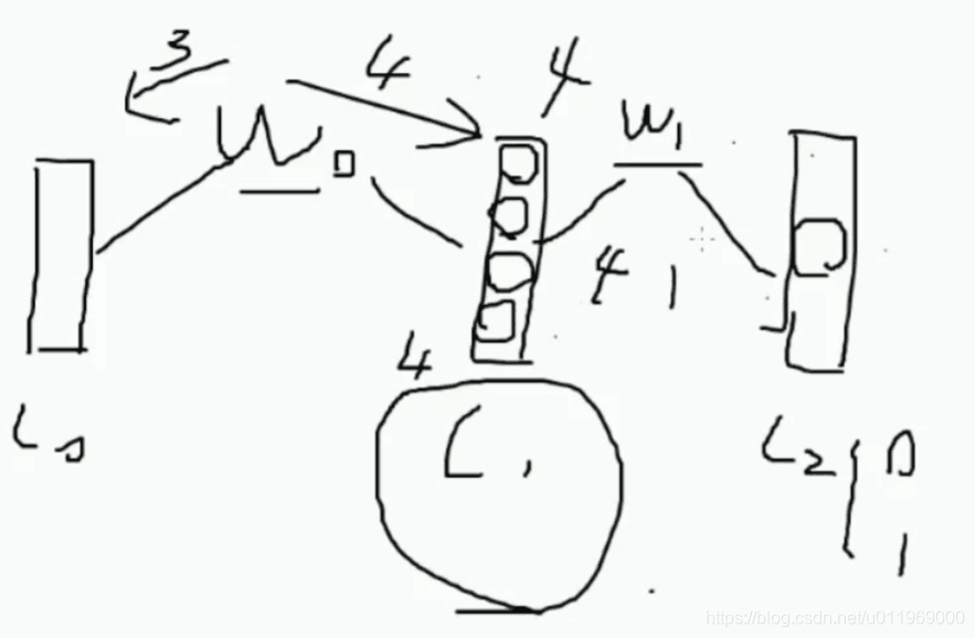
X0在输入层L0
LI为隐藏层
L2输出层
import numpy as np
#定义激活函数,前后项传播都需要经历激活函数
def sigmoid(x,deriv = False):#判断是否需要激活,需要激活则返回导数,不需要则返回原公式if (deriv == True):return x*(1-x)return 1/(1+np.exp(-x))
#指定输入x值,y值
#构造5个数据,每个数据有3个特征
x = np.array([[0,0,1],[0,1,1],[1,0,1],[1,1,1,],[0,0,1]])
#查看数据维度
print(x.shape)
#构造label,y值
y = np.array([[0],[1],[1],[0],[0]])
print(y.shape)
#指定随机种子
np.random.seed(1)
#参数的初始化,l0,l1,
w0 = np.random.random((3,4))
w1 = np.random.random((4,1))
print(w0,"\n **************\n",w1)
#随机的取值在-1到1之间
w0 = 2 * np.random.random((3,4)) - 1
w1 = 2 * np.random.random((4,1)) - 1
print(w0,"\n **************\n",w1)
#三层前向传播
for j in range(5):l0 = x #输入层l1 = sigmoid(np.dot(l0, w0)) #中间层l2 = sigmoid(np.dot(l1, w1)) #输出层l2_error = y - l2 #均方误差的求导后公式#print(l2_error.shape)if (j%6000) == 0:print('error' +str(np.mean(np.abs(l2_error))))#向前传播,l2_error越大说明错得越多,越需要更新权重#每个样本错了多少l2_delta = l2_error * sigmoid(12,deriv=True) #对应位置相乘#print(l2_error.shape) #5*1#print(l2_delta.shape) #5*1#print(w1.shape) #4*1l1_error = l2_delta.dot(w1.T)l1_delta = l1_error * sigmoid(11,deriv=True) #梯度更新参数权重,y-l2+=/l2-y-=/w1 += l1.T.dot(l2_delta)w0 += l0.T.dot(l1_delta)
目录 3-4感受神经网络的强大
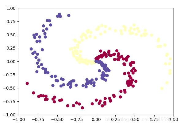
运行drawData脚本,随机输出3类点,每类100个,做三分类任务
import numpy as np
import matplotlib.pyplot as plt
plt.rcParams['figure.figsize'] = (10.0, 8.0) # set default size of plots
plt.rcParams['image.interpolation'] = 'nearest'
plt.rcParams['image.cmap'] = 'gray'
np.random.seed(0)
N = 100 # number of points per class
D = 2 # dimensionality
K = 3 # number of classes
X = np.zeros((N*K,D))
y = np.zeros(N*K, dtype='uint8')
for j in range(K):ix = range(N*j,N*(j+1))r = np.linspace(0.0,1,N) # radiust = np.linspace(j*4,(j+1)*4,N) + np.random.randn(N)*0.2 # thetaX[ix] = np.c_[r*np.sin(t), r*np.cos(t)]y[ix] = j
fig = plt.figure()
plt.scatter(X[:, 0], X[:, 1], c=y, s=40, cmap=plt.cm.Spectral)
plt.xlim([-1,1])
plt.ylim([-1,1])
plt.show()
数据呈环状的分不规则,通过线性无法切开,
对比1:使用线性分类,运行linerCla.py
#Train a Linear Classifier
import numpy as np
import matplotlib.pyplot as plt
np.random.seed(0)
N = 100 # number of points per class
D = 2 # dimensionality
K = 3 # number of classes
X = np.zeros((N*K,D))
y = np.zeros(N*K, dtype='uint8')
for j in range(K):ix = range(N*j,N*(j+1))r = np.linspace(0.0,1,N) # radiust = np.linspace(j*4,(j+1)*4,N) + np.random.randn(N)*0.2 # thetaX[ix] = np.c_[r*np.sin(t), r*np.cos(t)]y[ix] = j
# 初始化W和b
W = 0.01 * np.random.randn(D,K)
b = np.zeros((1,K))
# some hyperparameters,加入了正则化惩罚项
step_size = 1e-0
reg = 1e-3 # regularization strength
# gradient descent loop循环前后传播
num_examples = X.shape[0]
for i in range(1000):# evaluate class scores, [N x K]scores = np.dot(X, W) + b   #x:300*2 scores:300*3# compute the class probabilities,归一化操作exp_scores = np.exp(scores)probs = exp_scores / np.sum(exp_scores, axis=1, keepdims=True) # [N x K] probs:300*3#print(probs.shape) # compute the loss: average cross-entropy loss and regularization,计算出loss准备向前传播corect_logprobs = -np.log(probs[range(num_examples),y]) #corect_logprobs:300*1#print (corect_logprobs.shape)data_loss = np.sum(corect_logprobs)/num_examplesreg_loss = 0.5*reg*np.sum(W*W)loss = data_loss + reg_lossif i % 100 == 0:print ("iteration %d: loss %f" % (i, loss))# compute the gradient on scores,求解得出最好的模型参数dscores = probsdscores[range(num_examples),y] -= 1dscores /= num_examples# backpropate the gradient to the parameters (W,b)dW = np.dot(X.T, dscores)db = np.sum(dscores, axis=0, keepdims=True)dW += reg*W # regularization gradient# perform a parameter updateW += -step_size * dWb += -step_size * dbscores = np.dot(X, W) + b
predicted_class = np.argmax(scores, axis=1)
print ('training accuracy: %.2f' % (np.mean(predicted_class == y)))
h = 0.02
x_min, x_max = X[:, 0].min() - 1, X[:, 0].max() + 1
y_min, y_max = X[:, 1].min() - 1, X[:, 1].max() + 1
xx, yy = np.meshgrid(np.arange(x_min, x_max, h),np.arange(y_min, y_max, h))
Z = np.dot(np.c_[xx.ravel(), yy.ravel()], W) + b
Z = np.argmax(Z, axis=1)
Z = Z.reshape(xx.shape)
fig = plt.figure()
plt.contourf(xx, yy, Z, cmap=plt.cm.Spectral, alpha=0.8)
plt.scatter(X[:, 0], X[:, 1], c=y, s=40, cmap=plt.cm.Spectral)
plt.xlim(xx.min(), xx.max())
plt.ylim(yy.min(), yy.max())
plt.show()
输出结果
(base) D:\DL\02>E:/anaconda3/python.exe d:/DL/02/3-4class3NN/linerCla.py
iteration 0: loss 1.096919
iteration 100: loss 0.787937
iteration 200: loss 0.786281
iteration 300: loss 0.786231
iteration 400: loss 0.786230
iteration 500: loss 0.786230
iteration 600: loss 0.786230
iteration 700: loss 0.786230
iteration 800: loss 0.786230
iteration 900: loss 0.786230
training accuracy: 0.49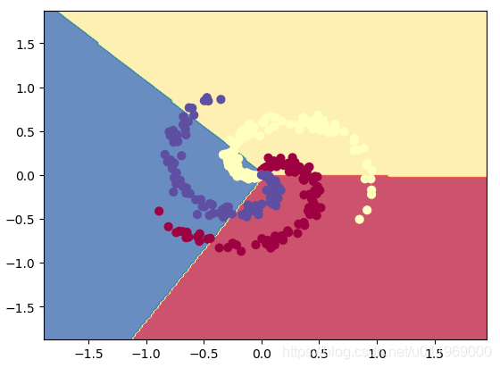
结论:线性分类器的表达效果不那么好
对比2:使用非线性分类,运行NNCla.py
import numpy as np
import matplotlib.pyplot as plt
np.random.seed(0)
N = 100 # number of points per class
D = 2 # dimensionality
K = 3 # number of classes
X = np.zeros((N*K,D))
y = np.zeros(N*K, dtype='uint8')
for j in range(K):ix = range(N*j,N*(j+1))r = np.linspace(0.0,1,N) # radiust = np.linspace(j*4,(j+1)*4,N) + np.random.randn(N)*0.2 # thetaX[ix] = np.c_[r*np.sin(t), r*np.cos(t)]y[ix] = jh = 100 # size of hidden layer,100个神经元
W = 0.01 * np.random.randn(D,h)# x:300*2  2*100
b = np.zeros((1,h))
W2 = 0.01 * np.random.randn(h,K)
b2 = np.zeros((1,K))
# some hyperparameters
step_size = 1e-0
reg = 1e-3 # regularization strength
# gradient descent loop
num_examples = X.shape[0]
for i in range(2000):# evaluate class scores, [N x K]hidden_layer = np.maximum(0, np.dot(X, W) + b) # note, ReLU activation hidden_layer:300*100#print hidden_layer.shapescores = np.dot(hidden_layer, W2) + b2  #scores:300*3#print scores.shape# compute the class probabilitiesexp_scores = np.exp(scores)probs = exp_scores / np.sum(exp_scores, axis=1, keepdims=True) # [N x K]#print probs.shape# compute the loss: average cross-entropy loss and regularizationcorect_logprobs = -np.log(probs[range(num_examples),y])data_loss = np.sum(corect_logprobs)/num_examplesreg_loss = 0.5*reg*np.sum(W*W) + 0.5*reg*np.sum(W2*W2)loss = data_loss + reg_lossif i % 100 == 0:print ("iteration %d: loss %f" % (i, loss))# compute the gradient on scoresdscores = probsdscores[range(num_examples),y] -= 1dscores /= num_examples# backpropate the gradient to the parameters# first backprop into parameters W2 and b2dW2 = np.dot(hidden_layer.T, dscores)db2 = np.sum(dscores, axis=0, keepdims=True)# next backprop into hidden layerdhidden = np.dot(dscores, W2.T)# backprop the ReLU non-linearitydhidden[hidden_layer <= 0] = 0# finally into W,bdW = np.dot(X.T, dhidden)db = np.sum(dhidden, axis=0, keepdims=True)# add regularization gradient contributiondW2 += reg * W2dW += reg * W# perform a parameter updateW += -step_size * dWb += -step_size * dbW2 += -step_size * dW2b2 += -step_size * db2
hidden_layer = np.maximum(0, np.dot(X, W) + b)
scores = np.dot(hidden_layer, W2) + b2
predicted_class = np.argmax(scores, axis=1)
print ('training accuracy: %.2f' % (np.mean(predicted_class == y)))h = 0.02
x_min, x_max = X[:, 0].min() - 1, X[:, 0].max() + 1
y_min, y_max = X[:, 1].min() - 1, X[:, 1].max() + 1
xx, yy = np.meshgrid(np.arange(x_min, x_max, h),np.arange(y_min, y_max, h))
Z = np.dot(np.maximum(0, np.dot(np.c_[xx.ravel(), yy.ravel()], W) + b), W2) + b2
Z = np.argmax(Z, axis=1)
Z = Z.reshape(xx.shape)
fig = plt.figure()
plt.contourf(xx, yy, Z, cmap=plt.cm.Spectral, alpha=0.8)
plt.scatter(X[:, 0], X[:, 1], c=y, s=40, cmap=plt.cm.Spectral)
plt.xlim(xx.min(), xx.max())
plt.ylim(yy.min(), yy.max())
plt.show()
(base) D:\DL\02>E:/anaconda3/python.exe d:/DL/02/3-4class3NN/NNCla.py
iteration 0: loss 1.098765
iteration 100: loss 0.723927
iteration 200: loss 0.697608
iteration 300: loss 0.587562
iteration 400: loss 0.426585
iteration 500: loss 0.357190
iteration 600: loss 0.349933
iteration 700: loss 0.346522
iteration 800: loss 0.336137
iteration 900: loss 0.309860
iteration 1000: loss 0.292278
iteration 1100: loss 0.284574
iteration 1200: loss 0.275849
iteration 1300: loss 0.271355
iteration 1400: loss 0.267756
iteration 1500: loss 0.265369
iteration 1600: loss 0.262948
iteration 1700: loss 0.260838
iteration 1800: loss 0.259226
iteration 1900: loss 0.257831
training accuracy: 0.97
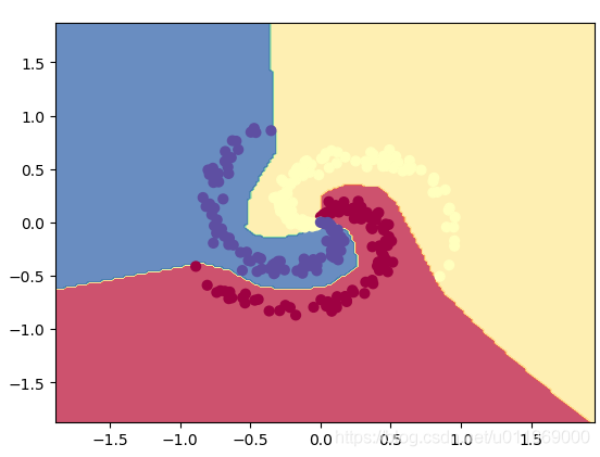
结论:适合非线性数据,缺点过拟合
3-5 神经网络案例-cifar分类任务
cifar数据集
The CIFAR-10 dataset consists of 60000 32x32 colour images in 10 classes, with 6000 images per class. There are 50000 training images and 10000 test images.
网页下载后,显示如下
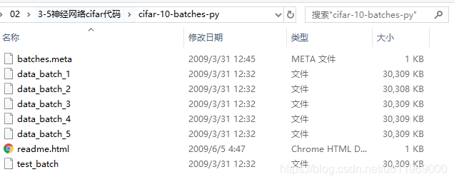
有5个batch,每个batch里面有1万张图片,
代码测试数据,在batch1取了,5000张训练图像,500张测试图像
Data_utils.py的get_CIFAR10_data函数进行了数据初始化
def get_CIFAR10_data(num_training=5000, num_validation=500, num_test=500):
数据是4维,h,w,c,b一次输入多张图像,一个batch一个batch进行迭代
1、读入数据集,切分数据,5000张训练数据,500验证数据,500测试集
验证集找到w 和b,再测试出测试集的label
2,神经网络网络结构
输入层data
中间层l1 +relu激活函数
输出层,output,10类别
使用softmax得出p1,p2,,,p10的10个类别的概率值
得出loss值反向传播算出w1和w2
3、规范的分模块写代码
3-6 神经网络案例-分模块构造神经网络
3-7 神经网络案例-训练神经网络完成
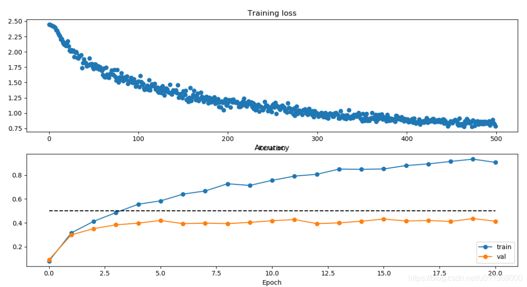
修改数据集路径,运行two_layer_fc_net_start.py
(tensorflow-gpu) D:\DL\02>E:/anaconda3/envs/tensorflow-gpu/python.exe d:/DL/02/3-5cifar-10-python/two_layer_fc_net_start.py
(10000, 32, 32, 3)
(Iteration 1 / 500) loss: 2.443408
(Epoch 0 / 40) train acc: 0.081000; val_acc: 0.092000
(Epoch 1 / 40) train acc: 0.316000; val_acc: 0.300000
(Epoch 2 / 40) train acc: 0.413000; val_acc: 0.352000
(Epoch 3 / 40) train acc: 0.486000; val_acc: 0.384000
(Epoch 4 / 40) train acc: 0.556000; val_acc: 0.398000
(Iteration 101 / 500) loss: 1.521124
(Epoch 5 / 40) train acc: 0.584000; val_acc: 0.420000
(Epoch 6 / 40) train acc: 0.640000; val_acc: 0.394000
(Epoch 7 / 40) train acc: 0.667000; val_acc: 0.398000
(Epoch 8 / 40) train acc: 0.727000; val_acc: 0.394000
(Iteration 201 / 500) loss: 1.160839
(Epoch 9 / 40) train acc: 0.713000; val_acc: 0.404000
(Epoch 10 / 40) train acc: 0.756000; val_acc: 0.418000
(Epoch 11 / 40) train acc: 0.791000; val_acc: 0.428000
(Epoch 12 / 40) train acc: 0.806000; val_acc: 0.394000
(Iteration 301 / 500) loss: 0.993981
(Epoch 13 / 40) train acc: 0.850000; val_acc: 0.400000
(Epoch 14 / 40) train acc: 0.848000; val_acc: 0.414000
(Epoch 15 / 40) train acc: 0.851000; val_acc: 0.432000
(Epoch 16 / 40) train acc: 0.879000; val_acc: 0.416000
(Iteration 401 / 500) loss: 0.901076
(Epoch 17 / 40) train acc: 0.893000; val_acc: 0.420000
(Epoch 18 / 40) train acc: 0.914000; val_acc: 0.412000
(Epoch 19 / 40) train acc: 0.933000; val_acc: 0.436000
(Epoch 20 / 40) train acc: 0.906000; val_acc: 0.414000
libpng warning: iCCP: cHRM chunk does not match sRGB
Validation set accuracy:  0.436
Test set accuracy:  0.386
结果
这篇关于深度学习入门(上)01(用cifar数据实现三层网络实现图片分类)的文章就介绍到这儿,希望我们推荐的文章对编程师们有所帮助!


