本文主要是介绍Image Recognition and Object Detection,希望对大家解决编程问题提供一定的参考价值,需要的开发者们随着小编来一起学习吧!
原文地址:https://www.learnopencv.com/image-recognition-and-object-detection-part1/
In this part, we will briefly explain image recognition using traditional computer vision techniques. I refer to techniques that are not Deep Learning based as traditional computer vision techniques because they are being quickly replaced by Deep Learning based techniques. That said, traditional computer vision approaches still power many applications. Many of these algorithms are also available in computer vision libraries like OpenCV and work very well out of the box.
A Brief History of Image Recognition and Object Detection
Our story begins in 2001; the year an efficient algorithm for face detection was invented by Paul Viola and Michael Jones. Their demo that showed faces being detected in real time on a webcam feed was the most stunning demonstration of computer vision and its potential at the time. Soon, it was implemented in OpenCV and face detection became synonymous with Viola and Jones algorithm.
Every few years a new idea comes along that forces people to pause and take note. In object detection, that idea came in 2005 with a paper by Navneet Dalal and Bill Triggs. Their feature descriptor, Histograms of Oriented Gradients (HOG), significantly outperformed existing algorithms in pedestrian detection.
Every decade or so a new idea comes along that is so effective and powerful that you abandon everything that came before it and wholeheartedly embrace it. Deep Learning is that idea of this decade. Deep Learning algorithms had been around for a long time, but they became mainstream in computer vision with its resounding success at the ImageNet Large Scale Visual Recognition Challenge (ILSVRC) of 2012. In that competition, an algorithm based on Deep Learning by Alex Krizhevsky, Ilya Sutskever, and Geoffrey Hinton shook the computer vision world with an astounding 85% accuracy — 11% better than the algorithm that won the second place! In ILSVRC 2012, this was the only Deep Learning based entry. In 2013, all winning entries were based on Deep Learning and in 2015 multiple Convolutional Neural Network (CNN) based algorithms surpassed the human recognition rate of 95%.
With such huge success in image recognition, Deep Learning based object detection was inevitable. Techniques like Faster R-CNN produce jaw-dropping results over multiple object classes. We will learn about these in later posts, but for now keep in mind that if you have not looked at Deep Learning based image recognition and object detection algorithms for your applications, you may be missing out on a huge opportunity to get better results.
With that overview, we are ready to return to the main goal of this post — understand image recognition using traditional computer vision techniques.
Image Recognition ( a.k.a Image Classification )
An image recognition algorithm ( a.k.a an image classifier ) takes an image ( or a patch of an image ) as input and outputs what the image contains. In other words, the output is a class label ( e.g. “cat”, “dog”, “table” etc. ). How does an image recognition algorithm know the contents of an image ? Well, you have to train the algorithm to learn the differences between different classes. If you want to find cats in images, you need to train an image recognition algorithm with thousands of images of cats and thousands of images of backgrounds that do not contain cats. Needless to say, this algorithm can only understand objects / classes it has learned.
To simplify things, in this post we will focus only on two-class (binary) classifiers. You may think that this is a very limiting assumption, but keep in mind that many popular object detectors ( e.g. face detector and pedestrian detector ) have a binary classifier under the hood. E.g. inside a face detector is an image classifier that says whether a patch of an image is a face or background.
Anatomy of an Image Classifier
The following diagram illustrates the steps involved in a traditional image classifier.
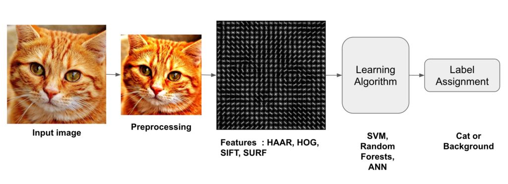
Interestingly, many traditional computer vision image classification algorithms follow this pipeline, while Deep Learning based algorithms bypass the feature extraction step completely. Let us look at these steps in more details.
Step 1 : Preprocessing
Often an input image is pre-processed to normalize contrast and brightness effects. A very common preprocessing step is to subtract the mean of image intensities and divide by the standard deviation. Sometimes, gamma correction produces slightly better results. While dealing with color images, a color space transformation ( e.g. RGB to LAB color space ) may help get better results.
Notice that I am not prescribing what pre-processing steps are good. The reason is that nobody knows in advance which of these preprocessing steps will produce good results. You try a few different ones and some might give slightly better results. Here is a paragraph from Dalal and Triggs
“We evaluated several input pixel representations including grayscale, RGB and LAB colour spaces optionally with power law (gamma) equalization. These normalizations have only a modest effect on performance, perhaps because the subsequent descriptor normalization achieves similar results. We do use colour information when available. RGB and LAB colour spaces give comparable results, but restricting to grayscale reduces performance by 1.5% at 10−4 FPPW. Square root gamma compression of each colour channel improves performance at low FPPW (by 1% at 10−4 FPPW) but log compression is too strong and worsens it by 2% at 10−4 FPPW.”
As you can see, they did not know in advance what pre-processing to use. They made reasonable guesses and used trial and error.
As part of pre-processing, an input image or patch of an image is also cropped and resized to a fixed size. This is essential because the next step, feature extraction, is performed on a fixed sized image.
Step 2 : Feature Extraction
The input image has too much extra information that is not necessary for classification. Therefore, the first step in image classification is to simplify the image by extracting the important information contained in the image and leaving out the rest. For example, if you want to find shirt and coat buttons in images, you will notice a significant variation in RGB pixel values. However, by running an edge detector on an image we can simplify the image. You can still easily discern the circular shape of the buttons in these edge images and so we can conclude that edge detection retains the essential information while throwing away non-essential information. The step is called feature extraction. In traditional computer vision approaches designing these features are crucial to the performance of the algorithm. Turns out we can do much better than simple edge detection and find features that are much more reliable. In our example of shirt and coat buttons, a good feature detector will not only capture the circular shape of the buttons but also information about how buttons are different from other circular objects like car tires.
Some well-known features used in computer vision are Haar-like featuresintroduced by Viola and Jones, Histogram of Oriented Gradients ( HOG ), Scale-Invariant Feature Transform ( SIFT ), Speeded Up Robust Feature ( SURF ) etc.
As a concrete example, let us look at feature extraction using Histogram of Oriented Gradients ( HOG ).
Histogram of Oriented Gradients ( HOG )
A feature extraction algorithm converts an image of fixed size to a feature vector of fixed size. In the case of pedestrian detection, the HOG feature descriptor is calculated for a 64×128 patch of an image and it returns a vector of size 3780. Notice that the original dimension of this image patch was 64 x 128 x 3 = 24,576 which is reduced to 3780 by the HOG descriptor.
HOG is based on the idea that local object appearance can be effectively described by the distribution ( histogram ) of edge directions ( oriented gradients ). The steps for calculating the HOG descriptor for a 64×128 image are listed below
- Gradient calculation : Calculate the x and the y gradient images,
and
, from the original image. This can be done by filtering the original image with the following kernels.

Using the gradient images and
, we can calculate the magnitude and orientation of the gradient using the following equations.

The calcuated gradients are “unsigned” and therefore is in the range 0 to 180 degrees.
2.Cells:Divide the image into 8×8 cells.
3.Calculate histogram of gradients in these 8×8 cells At each pixel in an 8×8 cell we know the gradient ( magnitude and direction ), and therefore we have 64 magnitudes and 64 directions — i.e. 128 numbers. Histogram of these gradients will provide a more useful and compact representation. We will next convert these 128 numbers into a 9-bin histogram ( i.e. 9 numbers ). The bins of the histogram correspond to gradients directions 0, 20, 40 … 160 degrees. Every pixel votes for either one or two bins in the histogram. If the direction of the gradient at a pixel is exactly 0, 20, 40 … or 160 degrees, a vote equal to the magnitude of the gradient is cast by the pixel into the bin. A pixel where the direction of the gradient is not exactly 0, 20, 40 … 160 degrees splits its vote among the two nearest bins based on the distance from the bin. E.g. A pixel where the magnitude of the gradient is 2 and the angle is 20 degrees will vote for the second bin with value 2. On the other hand, a pixel with gradient 2 and angle 30 will vote 1 for both the second bin ( corresponding to angle 20 ) and the third bin ( corresponding to angle 40 ).
4.Block normalization :The histogram calculated in the previous step is not very robust to lighting changes. Multiplying image intensities by a constant factor scales the histogram bin values as well. To counter these effects we can normalize the histogram — i.e. think of the histogram as a vector of 9 elements and divide each element by the magnitude of this vector. In the original HOG paper, this normalization is not done over the 8×8 cell that produced the histogram, but over 16×16 blocks. The idea is the same, but now instead of a 9 element vector you have a 36 element vector.
5.Feature Vector : In the previous steps we figured out how to calculate histogram over an 8×8 cell and then normalize it over a 16×16 block. To calcualte the final feature vector for the entire image, the 16×16 block is moved in steps of 8 ( i.e. 50% overlap with the previous block ) and the 36 numbers ( corresponding to 4 histograms in a 16×16 block ) calculated at each step are concatenated to produce the final feature vector.What is the length of the final vector ?
The input image is 64×128 pixels in size, and we are moving 8 pixels at a time. Therefore, we can make 7 steps in the horizontal direction and 15 steps in the vertical direction which adds up to 7 x 15 = 105 steps. At each step we calculated 36 numbers, which makes the length of the final vector 105 x 36 = 3780.
Step 3 : Learning Algorithm For Classification
In the previous section, we learned how to convert an image to a feature vector. In this section, we will learn how a classification algorithm takes this feature vector as input and outputs a class label ( e.g. cat or background ).
Before a classification algorithm can do its magic, we need to train it by showing thousands of examples of cats and backgrounds. Different learning algorithms learn differently, but the general principle is that learning algorithms treat feature vectors as points in higher dimensional space, and try to find planes / surfaces that partition the higher dimensional space in such a way that all examples belonging to the same class are on one side of the plane / surface.
To simplify things, let us look at one learning algorithm called Support Vector Machines ( SVM ) in some detail.
How does Support Vector Machine ( SVM ) Work For Image Classification?
Support Vector Machine ( SVM ) is one of the most popular supervised binary classification algorithm. Although the ideas used in SVM have been around since 1963, the current version was proposed in 1995 by Cortes and Vapnik.
In the previous step, we learned that the HOG descriptor of an image is a feature vector of length 3780. We can think of this vector as a point in a 3780-dimensional space. Visualizing higher dimensional space is impossible, so let us simplify things a bit and imagine the feature vector was just two dimensional.

In our simplified world, we now have 2D points representing the two classes ( e.g. cats and background ). In the image above, the two classes are represented by two different kinds of dots. All black dots belong to one class and the white dots belong to the other class. During training, we provide the algorithm with many examples from the two classes. In other words, we tell the algorithm the coordinates of the 2D dots and also whether the dot is black or white.
Different learning algorithms figure out how to separate these two classes in different ways. Linear SVM tries to find the best line that separates the two classes. In the figure above, H1, H2, and H3 are three lines in this 2D space. H1 does not separate the two classes and is therefore not a good classifier. H2 and H3 both separate the two classes, but intuitively it feels like H3 is a better classifier than H2 because H3 appears to separate the two classes more cleanly. Why ? Because H2 is too close to some of the black and white dots. On the other hand, H3 is chosen such that it is at a maximum distance from members of the two classes.
Given the 2D features in the above figure, SVM will find the line H3 for you. If you get a new 2D feature vector corresponding to an image the algorithm has never seen before, you can simply test which side of the line the point lies and assign it the appropriate class label. If your feature vectors are in 3D, SVM will find the appropriate plane that maximally separates the two classes. As you may have guessed, if your feature vector is in a 3780-dimensional space, SVM will find the appropriate hyperplane.
Optimizing SVM
So far so good, but I know you have one important unanswered question. What if the features belonging to the two classes are not separable using a hyperplane ? In such cases, SVM still finds the best hyperplane by solving an optimization problem that tries to increase the distance of the hyperplane from the two classes while trying to make sure many training examples are classified properly. This tradeoff is controlled by a parameter called C. When the value of C is small, a large margin hyperplane is chosen at the expense of a greater number of misclassifications. Conversely, when C is large, a smaller margin hyperplane is chosen that tries to classify many more examples correctly.
Now you may be confused as to what value you should choose for C. Choose the value that performs best on a validation set that the algorithm was not trained on.
这篇关于Image Recognition and Object Detection的文章就介绍到这儿,希望我们推荐的文章对编程师们有所帮助!


