CTPN源码解析3.1-model()函数解析

本文主要是介绍CTPN源码解析3.1-model()函数解析，希望对大家解决编程问题提供一定的参考价值，需要的开发者们随着小编来一起学习吧！

文本检测算法一：CTPN

CTPN源码解析1-数据预处理split_label.py

CTPN源码解析2-代码整体结构和框架

CTPN源码解析3.1-model()函数解析

CTPN源码解析3.2-loss()函数解析

CTPN源码解析4-损失函数

CTPN源码解析5-文本线构造算法构造文本行

CTPN训练自己的数据集

由于解析的这个CTPN代码是被banjin-xjy和eragonruan大神重新封装过的，所以代码整体结构非常的清晰，简洁！不像上次解析FasterRCNN的代码那样跳来跳去，没跳几步脑子就被跳乱了[捂脸]，向大神致敬！PS：里面肯定会有理解和注释错误的，欢迎批评指正！

解析源码地址：https://github.com/eragonruan/text-detection-ctpn

知乎：从代码实现的角度理解CTPN：https://zhuanlan.zhihu.com/p/49588885

知乎：理解文本检测网络CTPN：https://zhuanlan.zhihu.com/p/77883736

知乎：场景文字检测—CTPN原理与实现：https://zhuanlan.zhihu.com/p/34757009

 

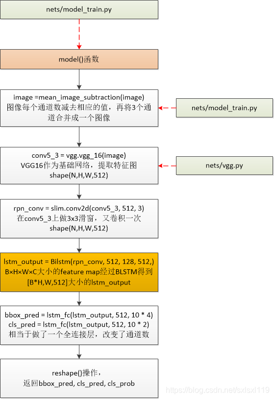
model()函数流程

model()函数代码

'''
0）传入图像，图像每个通道数减去相应的值，再将3个通道合并成一个图像
1）通过vgg16获得特征图conv5_3，shape(?,?,?,512)
2）滑动窗口获得特征向量rpn_conv，shape(?,?,?,512)
3）将得到的特征向量rpn_conv输入Bilstm中，得到lstm_output，shape(?,?,?,512)的输出
4）将lstm_output分别送入全连接层，得到 bbox_pred（预测框坐标）shape(?,?,?,40)，cls_pred(分类概率值) shape(?,?,?,20)。
5）shape转换，返回相应的值
'''
def model(image):image = mean_image_subtraction(image) #图像每个通道数减去相应的值，再将3个通道合并成一个图像with slim.arg_scope(vgg.vgg_arg_scope()):conv5_3 = vgg.vgg_16(image)  #nets/vgg.py,VGG16作为基础网络，提取特征图  shape(N,H,W,512)rpn_conv = slim.conv2d(conv5_3, 512, 3) #在conv5_3上做3x3滑窗，又卷积一次  shape(N,H,W,512)# B×H×W×C大小的feature map经过BLSTM得到[B*H,W,512]大小的lstm_outputlstm_output = Bilstm(rpn_conv, 512, 128, 512, scope_name='BiLSTM')  # shape(?,?,?,512)# 本代码做了调整：1.[B*H,W,512]大小的lstm_output没有接卷积层（FC代表卷积）# 2.[B*H,W,512]大小的lstm_output直接预测的四个回归量bbox_pred = lstm_fc(lstm_output, 512, 10 * 4, scope_name="bbox_pred") #网络预测回归输出  # shape(?,?,?,40)cls_pred = lstm_fc(lstm_output, 512, 10 * 2, scope_name="cls_pred")   #网络预测分类输出  # shape(?,?,?,20)# transpose: (1, H, W, A x d) -> (1, H, WxA, d)cls_pred_shape = tf.shape(cls_pred) # 将矩阵的维度输出为一个维度矩阵 shape(?,?,?,20)-> shape(4,?)cls_pred_reshape = tf.reshape(cls_pred, [cls_pred_shape[0], cls_pred_shape[1], -1, 2]) # shape(?,?,?,20)-># shape(?,?,?,2)cls_pred_reshape_shape = tf.shape(cls_pred_reshape) # 将矩阵的维度输出为一个维度矩阵 shape(?,?,?,2)-> shape(4,?)cls_prob = tf.reshape(tf.nn.softmax(tf.reshape(cls_pred_reshape, [-1, cls_pred_reshape_shape[3]])),[-1, cls_pred_reshape_shape[1], cls_pred_reshape_shape[2], cls_pred_reshape_shape[3]],name="cls_prob")  # shape(?,?,?,?)return bbox_pred, cls_pred, cls_prob

下面按model()函数的处理步骤分别解析源码

0）传入图像，图像每个通道数减去相应的值，再将3个通道合并成一个图像

这一步在model()函数中的执行语句是：

image = mean_image_subtraction(image) #图像每个通道数减去相应的值，再将3个通道合并成一个图像

'''
图像每个通道数减去相应的值，再将3个通道合并成一个图像
'''
def mean_image_subtraction(images, means=[123.68, 116.78, 103.94]):num_channels = images.get_shape().as_list()[-1]  #获取图像通道数if len(means) != num_channels:raise ValueError('len(means) must match the number of channels')channels = tf.split(axis=3, num_or_size_splits=num_channels, value=images)for i in range(num_channels):channels[i] -= means[i]  #图像每个通道数减去相应的值return tf.concat(axis=3, values=channels)  #再将3个通道合并成一个图像

1）通过vgg16获得特征图conv5_3，shape(?,?,?,512)

这一步在model()函数中的执行语句是：

rpn_conv = slim.conv2d(conv5_3, 512, 3) #在conv5_3上做3x3滑窗，又卷积一次  shape(N,H,W,512)

我就不贴vgg16卷积的代码了。

2）滑动窗口获得特征向量rpn_conv，shape(?,?,?,512)

这一步在model()函数中的执行语句是：

 rpn_conv = slim.conv2d(conv5_3, 512, 3) #在conv5_3上做3x3滑窗，又卷积一次  shape(N,H,W,512)

原意是结合该点周边9个点的信息，但在tensorflow中就用卷积代替了。

3）将得到的特征向量rpn_conv输入Bilstm中，得到lstm_output，shape(?,?,?,512)的输出

这一步在model()函数中的执行语句是：

# B×H×W×C大小的feature map经过BLSTM得到[B*H,W,512]大小的lstm_outputlstm_output = Bilstm(rpn_conv, 512, 128, 512, scope_name='BiLSTM')  # shape(?,?,?,512)

双向lstm获取横向（宽度方向）序列特征

'''
#BLSTM 双向LSTM
net,  特征图
input_channel,  输入的通道数 
hidden_unit_num, 隐藏层单元数目
output_channel,  输出的通道数
scope_name       #名称
'''
def Bilstm(net, input_channel, hidden_unit_num, output_channel, scope_name):# width--->time step  width方向作为序列方向with tf.variable_scope(scope_name) as scope:shape = tf.shape(net) #获取特征图的维度信息N, H, W, C = shape[0], shape[1], shape[2], shape[3]net = tf.reshape(net, [N * H, W, C])   # 改变数据格式  # shape(N * H, W, C)net.set_shape([None, None, input_channel])    # shape(?,?,input_channel)lstm_fw_cell = tf.contrib.rnn.LSTMCell(hidden_unit_num, state_is_tuple=True) #前向lstmlstm_bw_cell = tf.contrib.rnn.LSTMCell(hidden_unit_num, state_is_tuple=True) #反向lstmlstm_out, last_state = tf.nn.bidirectional_dynamic_rnn(lstm_fw_cell, lstm_bw_cell, net, dtype=tf.float32)lstm_out = tf.concat(lstm_out, axis=-1) # axis=1 代表在第1个维度拼接lstm_out = tf.reshape(lstm_out, [N * H * W, 2 * hidden_unit_num])# 这种初始化方法比常规高斯分布初始化、截断高斯分布初始化及 Xavier 初始化的泛化/缩放性能更好init_weights = tf.contrib.layers.variance_scaling_initializer(factor=0.01, mode='FAN_AVG', uniform=False)init_biases = tf.constant_initializer(0.0)weights = make_var('weights', [2 * hidden_unit_num, output_channel], init_weights)  # 初始化权重biases = make_var('biases', [output_channel], init_biases)  # 初始化偏移outputs = tf.matmul(lstm_out, weights) + biasesoutputs = tf.reshape(outputs, [N, H, W, output_channel]) #还原成原来的形状return outputs

4）将lstm_output分别送入全连接层，得到 bbox_pred（预测框坐标）shape(?,?,?,40)，cls_pred(分类概率值) shape(?,?,?,20)。

这一步在model()函数中的执行语句是：

    # 本代码做了调整：1.[B*H,W,512]大小的lstm_output没有接卷积层（FC代表卷积）# 2.[B*H,W,512]大小的lstm_output直接预测的四个回归量bbox_pred = lstm_fc(lstm_output, 512, 10 * 4, scope_name="bbox_pred") #网络预测回归输出  # shape(?,?,?,40)cls_pred = lstm_fc(lstm_output, 512, 10 * 2, scope_name="cls_pred")   #网络预测分类输出  # shape(?,?,?,20)

'''
全连接层，改变输出通道数
'''
def lstm_fc(net, input_channel, output_channel, scope_name):with tf.variable_scope(scope_name) as scope:shape = tf.shape(net)N, H, W, C = shape[0], shape[1], shape[2], shape[3]net = tf.reshape(net, [N * H * W, C])init_weights = tf.contrib.layers.variance_scaling_initializer(factor=0.01, mode='FAN_AVG', uniform=False)init_biases = tf.constant_initializer(0.0)weights = make_var('weights', [input_channel, output_channel], init_weights) #全连接层512-》output_channelbiases = make_var('biases', [output_channel], init_biases)output = tf.matmul(net, weights) + biasesoutput = tf.reshape(output, [N, H, W, output_channel])return output

5）shape转换，返回相应的值

这一步在model()函数中的执行语句是：

    # transpose: (1, H, W, A x d) -> (1, H, WxA, d)cls_pred_shape = tf.shape(cls_pred) # 将矩阵的维度输出为一个维度矩阵 shape(?,?,?,20)-> shape(4,?)cls_pred_reshape = tf.reshape(cls_pred, [cls_pred_shape[0], cls_pred_shape[1], -1, 2]) # shape(?,?,?,20)-># shape(?,?,?,2)cls_pred_reshape_shape = tf.shape(cls_pred_reshape) # 将矩阵的维度输出为一个维度矩阵 shape(?,?,?,2)-> shape(4,?)cls_prob = tf.reshape(tf.nn.softmax(tf.reshape(cls_pred_reshape, [-1, cls_pred_reshape_shape[3]])),[-1, cls_pred_reshape_shape[1], cls_pred_reshape_shape[2], cls_pred_reshape_shape[3]],name="cls_prob")  # shape(?,?,?,?)return bbox_pred, cls_pred, cls_prob

然后整个model()操作就结束了。

这篇关于CTPN源码解析3.1-model()函数解析的文章就介绍到这儿，希望我们推荐的文章对编程师们有所帮助！

---