Doing Math with Python读书笔记-第4章：Algebra and Symbolic Math with SymPy

本文主要是介绍Doing Math with Python读书笔记-第4章：Algebra and Symbolic Math with SymPy，希望对大家解决编程问题提供一定的参考价值，需要的开发者们随着小编来一起学习吧！

之前我们的操作都是使用数值，还有一种方式是使用符号，如x, y，我们称为符号数学。
我们使用SymPy库来实现书写表达式以及运算，安装如下：

$ pip3 install --user sympy

定义符号和符号操作

符号就是在代数和方程式中的变量。

>>> x=1; y=2
>>> 2*x + 3*y + 1
9

使用符号操作需要引入Symbol类，可以看到，现在x和y不用预先赋值了：

>>> from sympy import Symbol
>>> x = Symbol('x');  y = Symbol('y')
>>> 2*x + 3*y + 1
2*x + 3*y + 1

Symbol中的参数必须是字符串，表示变量名。
虽然变量的名字和符号的名字可以不一样，但建议一样：

>>> x.name;  y.name;
'x'
'y'
>>> abc = Symbol('x')
>>> abc.name
'x'
>>> type(abc)
<class 'sympy.core.symbol.Symbol'>

多个变量名赋值可采用以下简略形式：

>>> x,y,z = symbols('x,y,z')
>>> x.name, y.name, z.name
('x', 'y', 'z')

一些基本的运算会做展开，但复杂的不会：

>>> x + 2*x
3*x
>>> x*(2*x)
2*x**2
>>> x*(x + 2)	# 不会展开
x*(x + 2)

操作表达式

因式分解和展开表达式
因式分解(factorize )用factor()，展开用expand()。

>>> from sympy import Symbol, factor, expand
>>> x = Symbol('x')
>>> y = Symbol('y')
>>> factor(x**2 + 2*x + 1)	# 分解，x^2 + 2x +1 = (x + 1)^2
(x + 1)**2
>>> expand((x + 1)*(y + 1))	# 展开
x*y + x + y + 1
>>> expand(factor(x**2 + 2*x + 1))
x**2 + 2*x + 1

美化输出

>>> expr = x**2 + 2*x + 1
>>> print(expr)
x**2 + 2*x + 1
>>> from sympy import pprint
>>> pprint(expr)	# 没有想象中的美2          
x  + 2⋅x + 1

可以将表达式按升序排列，init_printing还有许多格式设定，详见帮助：

>>> from sympy import init_printing
>>> init_printing(order='rev-lex')
>>> expr2
1 + 2⋅x + x 
>>> expr = x**2/2
>>> expr2
x 
──
2 

代入变量

>>> expr = 2*x + y + 1
>>> expr
1 + y + 2⋅x 
>>> expr.subs({x:2, y:3})
8
>>> expr
1 + y + 2⋅x

更强大的是可以代入表达式：

>>> expr
1 + y + 2⋅x
>>> expr.subs({x:y})
1 + 3⋅y
>>> expr.subs({x:y-1})
-1 + 3⋅y
>>> expr.subs({x:2, y:x-1})	# 这个还不够聪明，因为是从左到右替代的
4 + x
>>> expr.subs({x:y+1, y:3})	# 写成这种方式就可以了
12

代入值的制定是通过字典数据类型，是键值对的集合。详见说明。
simplify()可以做合并等简化：

>>> from sympy import simplify>>> expr = x**2 + 2*x*y + y**2
>>> expr.subs({x:y-1})2                   2
(-1 + y)  + 2⋅y⋅(-1 + y) + y 
>>> sub = expr.subs({x:y-1})
>>> simplify(sub)2
1 - 4⋅y + 4⋅y 

以下是一个综合的示例，计算$x+\frac{x^2}{2}+\frac{x^3}{3}+\frac{x^4}{4}+...$

from sympy import Symbol, pprint, factor, expand, init_printingdef gen_expr(n):x = Symbol('x')e = xfor i in range(2, n+1):e += (x**i)/i result = e.subs({x:v})pprint(e)print(f'result is: {result}')return en = int(input('Enter the number of terms:'))
v = int(input('Enter the value of variable:'))
gen_expr(n)

运行：

$ p3 formula.py
Enter the number of terms:4
Enter the value of variable:24    3    2    
x    x    x     
── + ── + ── + x
4    3    2     
result is: 32/3

很奇怪，以下的代码运行失败：

from sympy import Symbol, pprint, factor, expand, init_printingdef gen_expr(n):x = Symbol('x')e = xfor i in range(2, n+1):e += (x**i)/i return en = int(input('Enter the number of terms:'))
v = int(input('Enter the value of variable:'))
expr = gen_expr(n)
result = expr.subs({x:v})
print(f'result is: {result}')

运行：

$ p3 formula.py
Enter the number of terms:4
Enter the value of variable:2
Traceback (most recent call last):File "formula.py", line 15, in <module>result = expr.subs({x:v})
NameError: name 'x' is not defined

改成一下就好了，看来还是变量范围的问题：

from sympy import Symbol, pprint, factor, expand, init_printingx = Symbol('x')def gen_expr(n):e = xfor i in range(2, n+1):e += (x**i)/ireturn en = int(input('Enter the number of terms:'))
v = int(input('Enter the value of variable:'))
expr = gen_expr(n)
result = expr.subs({x:v})
print(f'result is: {result}')

将字符串转换为数学表达式

>>> from sympy import sympify
>>> expr = 'x**2 + 2*x + 1'
>>> expr = sympify(expr)
>>> expr2
1 + 2⋅x + x 
>>> type(expr)
<class 'sympy.core.add.Add'>
>>> expr * expr2
⎛           2⎞ 
⎝1 + 2⋅x + x ⎠ 
>>> 2 * expr2
2 + 4⋅x + 2⋅x 

注意输入必须是有效的，否则抛出SympifyError异常。例如2*x不能写成2x。
sympify有个明显的好处，就是不用预先定义Symbol了：

>>> from sympy import Symbol, sympify
>>> expr1 = sympify('x + 1')
>>> expr2 = sympify('y + 1')
>>> expr3 = expr1 * expr2
>>> expr2
1 + y
>>> expr3
(1 + x)⋅(1 + y)
>>> expand(expr3)
1 + y + x + x⋅y

解方程

使用solve()，其总是假设表达式等于0：

>>> from sympy import Symbol, sympify, solve
>>> expr = sympify('x**2 + 2*x + 1')
>>> expr2
1 + 2⋅x + x 
>>> solve(expr)
[-1]
>>> expr = sympify('(x + 1)*(y -1)')
>>> solve(expr)
[{x: -1}, {y: 1}]

解二次方程
二次方程（Quadratic Equations）。以下方程有多个解：

>>> expr = sympify('x**2 + 5*x + 4')
>>> solve(expr)
[-4, -1]

复数方程式也可以解：

>>> x=Symbol('x')
>>> expr = x**2 + x + 1
>>> solve(expr)				# i表示虚数，是-1的平方根（imaginary）
⎡  √3⋅ⅈ   1  √3⋅ⅈ   1⎤
⎢- ──── - ─, ──── - ─⎥
⎣   2     2   2     2⎦
>>> solve(expr, dict=True)	# 字典形式
⎡⎧     √3⋅ⅈ   1⎫  ⎧   √3⋅ⅈ   1⎫⎤
⎢⎨x: - ──── - ─⎬, ⎨x: ──── - ─⎬⎥
⎣⎩      2     2⎭  ⎩    2     2⎭⎦

也可以只求解一个变量，这个变量用其余的变量表示，注意solve()中多指定了一个参数：

>>> a=Symbol('a')
>>> b=Symbol('b')
>>> x=Symbol('x')
>>> expr = a*x**2 + b*x + 1
>>> solve(expr, x)
⎡   __________       ⎛   __________    ⎞ ⎤
⎢  ╱  2              ⎜  ╱  2           ⎟ ⎥
⎢╲╱  b  - 4⋅a  - b  -⎝╲╱  b  - 4⋅a  + b⎠ ⎥
⎢─────────────────, ─────────────────────⎥
⎣       2⋅a                  2⋅a         ⎦

作者给了个运动方程式(equations of motion)的例子，其中a是加速度，t是时间，$\mu$是速度，s是距离：
$s=\mu t+\frac{1}{2}a{t}^2$
可以计算下距离一定时所需的时间。

解线性方程组

>>> x = Symbol('x')
>>> y = Symbol('y')
>>> expr1 = x + 3*y - 11
>>> expr2 = x - 2*y - 1
>>> solve((expr1, expr2))
{x: 5, y: 2}

以下是验算过程：

>>> sol = solve((expr1, expr2), dict=True)
>>> sol[0]
{x: 5, y: 2}
>>> sol[0][x]
5
>>> sol[0][y]
2
>>> expr1.subs({x:5, y:2})
0
>>> expr2.subs({x:5, y:2})
0

使用SYMPY绘图

在前面的章节，我们用matplotlib绘图，但必须指定x和y的值。而使用sympy绘图，只需给出公式就可以了。

>>> from sympy.plotting import plot
>>> from sympy import Symbol
>>> x = Symbol('x')
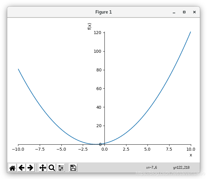
>>> plot(x**2 + 2*x + 1)Plot object containing:                   
[0]: cartesian line: x**2 + 2*x + 1 for x over (-10.0, 10.0)
>>> plot((x**2 + 2*x + 1), (x, -100, 100))	# 可指定x的取值区间Plot object containing:                    
[0]: cartesian line: x**2 + 2*x + 1 for x over (-100.0, 100.0)

第一个输出如下：

指定标题与标签：

>>> plot(x**2 + 2*x + 1, title='A Line', xlabel='x', ylabel='2x+3')

不显示，仅存为文件：

>>> p = plot(x**2 + 2*x + 1, show = False)
>>> p.save('f.png')

绘制用户输入的表达式

1. 用户输入的表达式有两个变量x和y，通过sympify()转换为符号表达式，
2. 通过solve(表达式, y)得到x和y的关系
3. 通过plot()绘图

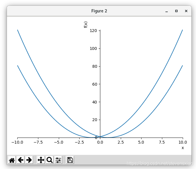
绘制多个函数

>>> plot(x**2 + 2*x + 1, x**2 - 2*x + 1)

调用plot()时，默认程序会阻塞，直到图形关闭。以下是一种延后到show()调用时阻塞的方法：

>>> p=plot(x**2 + 2*x + 1, x**2 - 2*x + 1, show=False)
>>> pPlot object containing:                   
[0]: cartesian line: x**2 + 2*x + 1 for x over (-10.0, 10.0)
[1]: cartesian line: x**2 - 2*x + 1 for x over (-10.0, 10.0)
>>> p[0].line_color = 'r'	# 红色线
>>> p[1].line_color = 'b'	# 蓝色线
>>> p.legend = True
>>> p.show()

编程挑战

因式分解
用户输入表达式，然后做因式分解：

>>> x = Symbol('x')
>>> expr = x**3 + 3*x**2 + 3*x + 1
>>> factor(expr)3
(1 + x) 

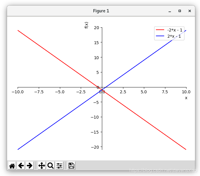
二元一次方程绘图
代码：

from sympy import Symbol, sympify, solve
from sympy.plotting import plotexpr1 = input('Enter your first expression in terms of x and y: ')
expr2 = input('Enter your second expression in terms of x and y: ')sol1 = solve(expr1, 'y')	# solve()也可以接受字符串，不仅仅是符号表达式
sol2 = solve(expr2, 'y')p = plot(sol1[0], sol2[0], show=False)
p[0].line_color = 'r'	
p[1].line_color = 'b'
p.legend = True
p.show()

输出：

$ p3 eqplot.py
Enter your first expression in terms of x and y: y + 2*x + 1
Enter your second expression in terms of x and y: y - 2*x + 1

序列求和
$\sum _{x=1}^{10}\frac{1}{x}$

>>> from sympy import Symbol, summation, pprint
>>> x = Symbol('x')
>>> s = summation(1/x, (x, 1, 10))
>>> s
7381
────
2520

又如:
$\sum _{n=1}^{10}\frac{x^n}{n}$

>>> x = Symbol('x')
>>> n = Symbol('n')
>>> s = summation(x**n/n, (n, 1, 10))
>>> s2    3    4    5    6    7    8    9    10x    x    x    x    x    x    x    x    x  
x + ── + ── + ── + ── + ── + ── + ── + ── + ───2    3    4    5    6    7    8    9     10
>>> s.subs({x:1})
7381
────
2520

单变量不等式
solve()也支持不等式的求解，支持的不等式类型包括多项式(polynomial)，有理式(rational expression)。
先来看多项式。多项式中只有一个变量，只有加减乘操作，幂都是正数。

>>> from sympy import Poly, Symbol, solve_poly_inequality
>>> x = Symbol('x')
>>> ineq_obj = x**2 -4 > 0
>>> lhs = ineq_obj.lhs		# 提取不等式左边部分
>>> lhs2
-4 + x 
>>> p = Poly(lhs, x)
>>> p
Poly(x**2 - 4, x, domain='ZZ')
>>> rel = ineq_obj.rel_op	# 提取操作符
>>> rel
>
>>> solve_poly_inequality(p, rel)
[(-∞, -2), (2, ∞)]

再来看有理式，也称为分式。有理式的分子和分母都是多项式。

>>> from sympy import Symbol, Poly, solve_rational_inequalities
>>> x = Symbol('x')
>>> ineq_obj = ((x-1)/(x+2)) > 0
>>> lhs = ineq_obj.lhs
>>> lhs
-1 + x
──────
2 + x 
>>> numer, denom = lhs.as_numer_denom()
>>> numer	# 分子(numerator)
-1 + x
>>> denom	# 分母(Denominator)
2 + x
>>> p1 = Poly(numer)
>>> p1
Poly(x - 1, x, domain='ZZ')
>>> p2 = Poly(denom)
>>> p2
Poly(x + 2, x, domain='ZZ')
>>> rel = ineq_obj.rel_op
>>> solve_rational_inequalities([[((p1, p2), rel)]])
(-∞, -2) ∪ (1, ∞)

最后看一下其它类型的不等式，例如sin(x) - 0.6 > 0：

>>> from sympy import Symbol, solve, solve_univariate_inequality, sin
>>> x = Symbol('x')
>>> ineq_obj = sin(x) - 0.6 > 0
>>> solve_univariate_inequality(ineq_obj, x, relational=False)
(0.643501108793284, π - 0.643501108793284)

is_polynomial()可以检测表达式是否为多项式。

>>> x = Symbol('x')
>>> expr = x**2 + 2*x + 1
>>> expr.is_polynomial()
True
>>> expr = sin(x)
>>> expr.is_polynomial()
False

is_rational_function()可判断表达式是否为有理式。
sympify()也可以将不等式字符串转换为表达式。

这篇关于Doing Math with Python读书笔记-第4章：Algebra and Symbolic Math with SymPy的文章就介绍到这儿，希望我们推荐的文章对编程师们有所帮助！

---