远场Far-Field beamforming与近场Near-Field beamforming有何关系

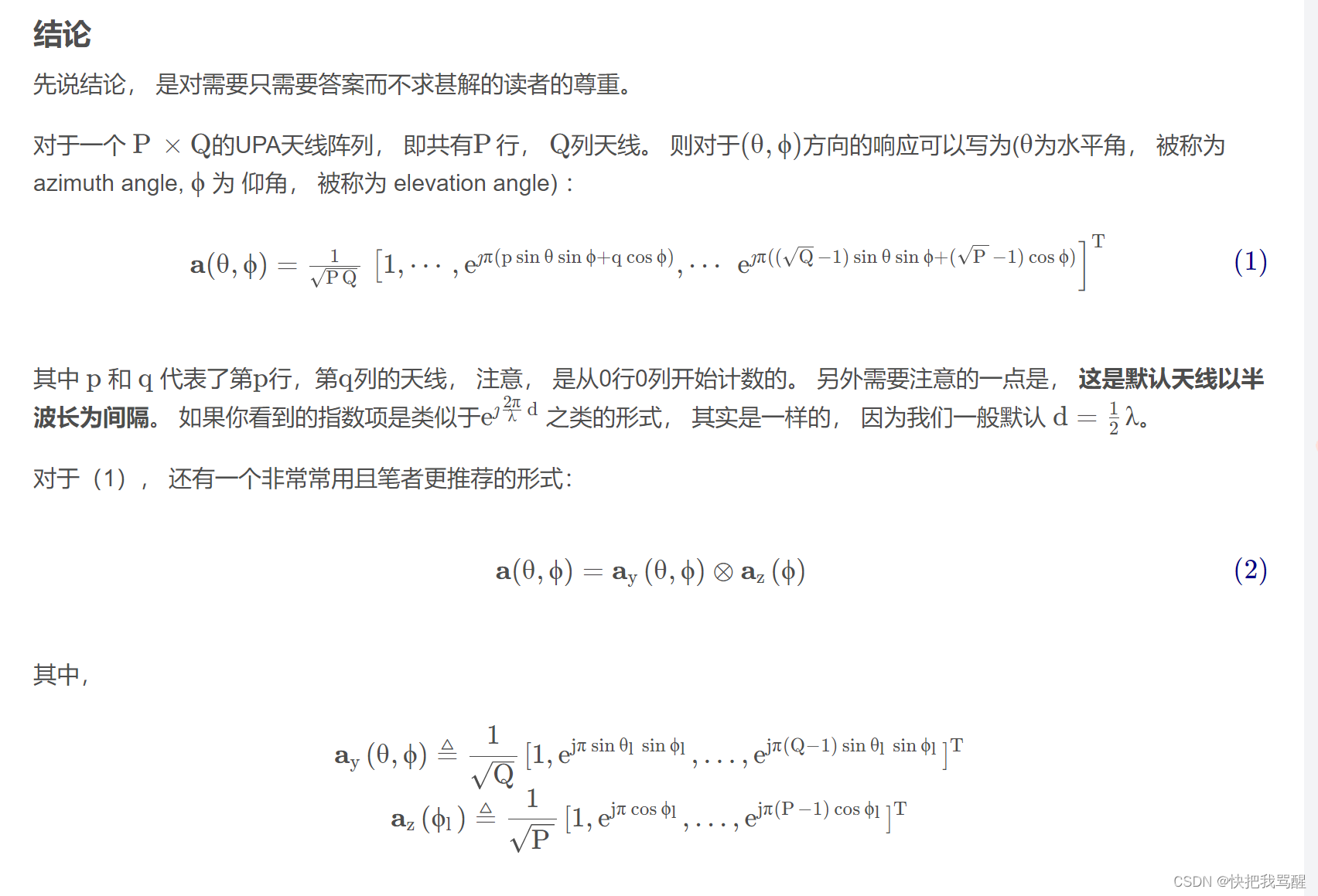
UPA

写在前面

Dai Linglong老师的简介网站

Channel Estimation for Extremely Large-Scale Massive MIMO:Far-Field, Near-Field, or Hybrid-Field?

近场的方向向量，把里边每一项做泰勒展开，如果把高阶项近似为0，则为远场。近场是保留了二阶小量，然后远场是只保留一阶小量。

信道估计： 已知发射端发射导频和接收端的接收导频信号估计信道。
$N$ BS处天线数
$D$ 天线孔径
$\lambda$ 天线波长
瑞利距离$Z$：$Z=2D^2/\lambda$

Far Field model

1. Far-Field Channel Model: As shown in Fig. 1, when the distance between the BS and the scatter is larger than the Rayleigh distance, the far-field channel ${\mathbf{h}}_{\text{far-field }}$ is modeled under the planar wave assumption, which can be represented by

$${\mathbf{h}}_{\text{far-field }}=\sqrt{\frac{N}{L}}\sum _{l=1}^L{\alpha }_l\mathbf{a}\left({\theta }_l\right)\text{\hspace{1em}(3)}$$

where $L$ represents the number of path components (corresponding to effective scatters) between the BS and the user, ${\alpha }_l$ and ${\theta }_l$ represent the gain and angle for the $l$th path, respectively. a $\left({\theta }_l\right)$ represents the far-field array steering vector based on the planar wave assumption, which can represented by`

$$\mathbf{a}\left({\theta }_l\right)=\frac{1}{\sqrt{N}}{\left[1,e^{-j\pi {\theta }_l},\dots ,e^{-j(N-1)\pi {\theta }_l}\right]}^H\text{\hspace{1em}(4)}$$

It is noted that ${\theta }_l=2\frac{d}{\lambda }\cos \left({\varphi }_l\right)$ , where $d=\frac{\lambda }{2}$ is the antenna spacing, and ${\varphi }_l\in (0,\pi )$ is the practical physical angle.

In order to reduce the pilot overhead for the channel estimation, the above non-sparse channel ${\mathbf{h}}_{\text{far-field }}$ can be represented by the sparse angle-domain channel ${\mathbf{h}}_{\text{far-field }}^A$ with the DFT matrix $\mathbf{F}$ as follows

$${\mathbf{h}}_{\text{far-field }}=\mathbf{F}{\mathbf{h}}_{\text{far-field }}^A\text{\hspace{1em}(5)}$$

where $\mathbf{F}=\left[\mathbf{a}\left({\theta }_1\right),\dots ,\mathbf{a}\left({\theta }_N\right)\right]$ is a $N$ \times $N$ unitary matrix, where the columns are orthogonal to each other, and ${\theta }_n=\frac{2n-N-1}{N}$ with $n=1,2,\dots ,N$ . Since there are limited scatters in communication environments, the angle-domain channel ${\mathbf{h}}_{\text{far-field }}^A$ is usually sparse. Based on this sparsity, some CS algorithms can be used to estimate this high-dimensional channel with low pilot overhead [3]-[5].

Near Field model

除了上述远场信道模型之外，最近在[6]中提出了近场信道模型。如图1所示，当基站与散射体之间的距离小于瑞利距离时，近场信道在球面波假设下建模，可以表示为

$${\mathbf{h}}_{\text{near-field }}=\sqrt{\frac{N}{L}}\sum _{l=1}^L{\alpha }_l\mathbf{b}\left({\theta }_l,r_l\right)\text{\hspace{1em}(6)}$$

与远场信道模型（3）相比，基于球面波假设推导了近场信道模型的阵列导向矢量$\mathbf{b}\left({\theta }_l,r_l\right)$，可以表示为[6]

$$\mathbf{b}\left({\theta }_l,r_l\right)=\frac{1}{\sqrt{N}}{\left[e^{-j\frac{2\pi }{\lambda }\left(r_l^{(1)}-r_l\right)},\dots ,e^{-j\frac{2\pi }{\lambda }\left(r_l^{(N)}-r_l\right)}\right]}^H\text{\hspace{1em}(7)}$$

where $r_l$ represents the distance from the $l$ th scatter to the center of the antenna array, $r_l^{(n)}=\sqrt{r_l^2+{\delta }_n^2{d}^2-2r_l{\delta }_{n}d{\theta }_l}$ represents the distance from the $l$ th scatter to the $n$ th BS antenna, and ${\delta }_n=\frac{2n-N-1}{2}$ with $n=1,2,\dots ,N$ .

Since the DFT matrix in (5) associated with the angle domain only matches the array steering vector in the far-field, the near-field channel in (6) will cause serious energy spread in angle domain. In order to explore the sparsity of the near-field channel, a polar-domain transform matrix $\mathbf{W}$ was proposed in [6], which can be represented by (为了探索近场信道的稀疏性，极化域变换矩阵$\mathbf{W}$)

$$\begin{array}{r}\mathbf{W}=[\mathbf{b}\left({\theta }_1,r_1^1\right),\dots ,\mathbf{b}\left({\theta }_1,r_1^{S_1}\right),\dots ,\\ \mathbf{b}\left({\theta }_N,r_N^1\right),\dots ,\mathbf{b}\left({\theta }_N,r_N^{S_N}\right)]\end{array}\text{\hspace{1em}(8)}$$

where each column of $\mathbf{W}$ is a near-field array steering vector with the sampled angle ${\theta }_n$ and distance $r_n^{s_n}$ , with $s_n=1,2,\dots ,S_n$, $S_n$ represents the number of sampled distances at the sampled angle ${\theta }_n$ . Thus, the number of all sampled grids can be represented by $S={\sum }_{n=1}^N{S}_n$ . Based on this polar-domain transform matrix $\mathbf{W}$ , the near-field channel can be represented by

近场把信道变换到极化域（在极化域中信道是稀疏的）

$${\mathbf{h}}_{\text{near-field }}=\mathbf{W}{\mathbf{h}}_{\text{near-field }}^P\text{\hspace{1em}(9)}$$

where ${\mathbf{h}}_{\text{near-field }}^P$ is the $S\times 1$ polar-domain channel. Similar to the far-field channel in the angle domain, ${\mathbf{h}}_{\text{near-field }}^P$ also shows a certain sparsity. The corresponding polar-domain based CS algorithm was further proposed to reduce the pilot overhead for the near-field channel estimation [6]. However, since the polar transform matrix $\mathbf{W}$ is generated from the joint angle and distance space, its dimension is large, and the columns orthogonality is relatively poor compared with the DFT matrix. Thus, the far-field channel in the polar domain may cause more serious energy leakage than that in the angle domain.

极化域的远场通道可能比角域的远场通道造成更严重的能量泄漏。

在上述所有现有工作中，通信环境中的所有散射都假设位于远场或近场区域。在实际的XL-MIMO通信环境中，更有可能一些散射位于远场区域，而另一些则可能位于近场区域。然而，这种混合场通信环境无法通过现有的远场或近场信道模型来精确建模，因此现有的远场和近场信道估计方案不能直接用于精确估计混合场XL- MIMO 信道。

Multi-Beam Design for Near-Field Extremely Large-Scale RIS-Aided Wireless Communications

abstract

可重构智能表面（RIS）作为由无源元件组成的节能阵列，将向超大规模RIS（XL-RIS）发展，以克服严重的路径损耗。这种变化导致近场传播成为主导。有一些工作探索通过波束训练来设计近场波束。不幸的是，由于XL-RIS的恒模约束，在近场场景中的大多数工作集中在单波束设计。对于大规模连接需求的场景，这些工作将面临严重的波束增益损失，导致传输速率下降。为了解决这个问题，我们提出了一个块坐标下降为基础的计划与优化最小化（MM）算法的多波束设计。该方案从两个方面处理常数模约束。首先，在此约束下，多波束设计是一个棘手的非凸二次规划问题。我们利用MM算法来解决这个问题的几个迭代的子问题，很容易解决。其次，多波束优化的解空间被限制在一个有限的空间，由于这种约束，所以我们引入波束增益相位作为一个额外的优化变量，以丰富优化的自由度。仿真结果表明，该方案比现有方案提高了50%的速率。

intro

可重构智能表面（RIS）被认为是未来无线通信最有前途的技术之一[2]，[3]。RIS被赋予通过创建可控反射链路来操纵信号传播环境的能力[4]、[5]。受益于这种能力，RIS有望带来克服阻塞[6]，[7]，确保安全传输[8]，增强覆盖[9]，[10]以及提高频谱效率[11]，[12]的潜在优势。

然而，由于实际无线系统中的乘法衰落效应，RIS的期望性能将受到严重限制[13]、[14]。由于发射机-RIS-接收机反射链路的严重路径损耗是发射机-RIS链路和RIS-接收机链路的路径损耗的乘积（而不是总和）。考虑到RIS的阵列增益与RIS元件数量的平方成比例[14]，[15]，这种严重的乘法路径损耗可以通过使用大量低成本RIS元件扩大阵列孔径来有效补偿[6]，[16]。因此，RIS的演进可能会朝着用于未来无线网络的超大规模RIS（XL-RIS）发展[17]。

为了探索XL-RIS的潜在性能**，重要的是根据准确的信道状态信息（CSI）来设计RIS波束成形**。随着RIS元素数量的增加，由于计算复杂度高，估计完美的CSI是相当困难的。作为另一种方案，许多工作设计波束形成而不需要精确的CSI。具体地，指向期望空间角度的波束将通过波束训练从预先设计的码本中选择。这些工作对于现有RIS系统是有效的。然而，随着RIS阵列孔径的增大，其电磁辐射特征将从现有的远场平面波前演变为近场球面波前。为了保证波束成形性能，波束不仅要在角度域进行调整，而且还要在距离域进行调整，现有的工作已经不再有效。因此，探索XL-RIS辅助无线通信的近场波束设计是至关重要的。

Contribution

为了提高最小速率，我们研究了XL-RIS的近场多波束设计，以服务于多个用户。本文的具体贡献可归纳如下。

首先，与现有的单用户近场单波束设计方法不同，本文提出了一种适用于近场XL-RIS波束形成的多波束设计方法。该方法的核心目标是在恒模约束下从XL-RIS中生成指向用户期望区域的近场多波束，并具有期望的波束增益。该方法由波束训练和多波束设计两部分组成。第一个过程由所有用户独立执行，以获取每个用户的期望单波束方向。然后，多波束设计过程被制定为一个非凸二次规划，以获得波束形成向量，其中的规划目标，是由第一个程序获得。

其次，为了解决非凸二次规划，我们提出了一个块坐标下降（BCD）的方案与优化最小化（MM）算法来实现多波束设计过程。该方案从两个方面处理了恒模约束的影响。首先，在此约束下，多波束设计问题是一个棘手的非凸优化问题。因此，我们解决棘手的问题，分解成一系列易于处理的子问题迭代解决的帮助下的MM算法。然后，注意到多波束设计的解空间是不完整的，由于常数模约束，我们引入初始优化目标的相位信息作为额外的可优化变量。因此，可以丰富优化的自由度。最后，我们执行波束的设计程序，通过BCD策略交替优化以上两个方面。此外，还给出了每次迭代的封闭解。

仿真结果表明，所提出的近场多波束设计可以实现最小速率的所有用户比现有的近场计划高50%。特别是，我们还进行了远场用户的模拟，这表明该方案也有一个性能增益相比，现有的远场单波束设计方案。

system model

在这一部分中，首先给出了XL-RIS辅助无线通信的信号模型，在此基础上分别给出了远场和近场情况下的信道模型。

信号模型

在这一部分中，首先给出了XL-RIS辅助无线通信的信号模型，在此基础上分别给出了远场和近场情况下的信道模型。

Signal Model

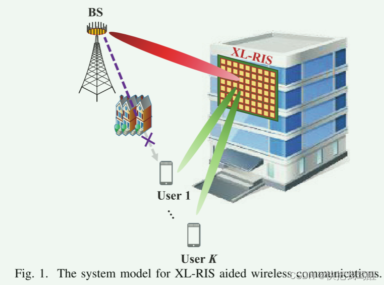
We consider an XL-RIS aided wireless communications, as illustrated in Fig. 1, where a base station (BS) with $M$ antennas assisted by an XL-RIS with $N$ elements simultaneously serves $K$ single-antenna users. Let N = { 1 , 2 , ⋯ , N } \mathcal{N}=\{1,2, \cdots, N\} N={1,2,⋯,N} and K = { 1 , 2 , ⋯ , K } \mathcal{K}=\{1,2, \cdots, K\} K={1,2,⋯,K} denote the index sets of XL-RIS elements and users, respectively. The uniform linear array (ULA) of antennas is employed at the BS, and the uniform planar array (UPA) of elements is employed at the XL-RIS [33]. We consider that the XL-RIS is deployed with $N_1$ horizontal rows and $N_2$ vertical columns $\left(N=N_1\times N_2\right)$ . We adopt the assumption that the direct BS-user transmission link is blocked by the obstacles [26], [34]. For the $k$ th user with $k\in \mathcal{K}$ , the received signal $y_k$ can be expressed as

$$y_k={\mathbf{h}}_{r,k}^T\mathbf{\Theta }\mathbf{Gx}+n_k\text{\hspace{1em}(1)}$$

where $\mathbf{x}\in {\mathbb{C}}^{M\times 1}$ is the precoded transmitted signal at the BS; ${\mathbf{h}}_{r,k}^T\in {\mathbb{C}}^{1\times N}$ , and $\mathbf{G}\in {\mathbb{C}}^{N\times M}$ denote the RIS-user channel from the XL-RIS to the $k$ th user, and the BS-RIS channel from the BS to the XL-RIS, respectively; $\Theta \in {\mathbb{C}}^{N\times N}$ represents the beamforming matrix of the XL-RIS; $n_k\sim \mathcal{C}\mathcal{N}\left(0,{\sigma }_n^2\right)$ denotes the additive white Gaussian noise (AWGN) received at the $k$ th user.

The XL-RIS composed of extremely large number of passive reflecting elements can adjust the phase of a incident signal by designing $\Theta$ as

$$\mathbf{\Theta }\triangleq \mathrm{diag}(\mathbf{\theta })=\mathrm{diag}\left({\theta }_1,\cdots ,{\theta }_n,\cdots ,{\theta }_N\right)\text{\hspace{1em}(2)}$$

where $\mathbf{\theta }$ respresents the RIS beamforming vector, ${\theta }_n=e^{j{p}_n}\left(p_n\in [0,2\pi ],n\in \mathcal{N}\right)$ represents the reflecting coefficient of the $n$ th XL-RIS element.

According to (2), the received signal model in (1) can be rewritten as

$$y_k={\mathbf{\theta }}^T\mathrm{diag}\left({\mathbf{h}}_{r,k}^T\right)\mathbf{Gx}+n_k\text{\hspace{1em}(3)}$$

where the reflecting channel for the $k$ th user is defined as $\mathbf{H}=\mathrm{diag}\left({\mathbf{h}}_{r,k}^T\right)\mathbf{G}$ . Then, we will introduce the channel model in the far-field scenario and the near-field scenario, respectively.

---

---

远场信道模型

在给出XL-RIS辅助无线通信的近场信道模型之前，我们首先介绍了现有的远场信道模型，该模型在当前的研究中得到了广泛的考虑。考虑到用于高频传输的几何信道模型[35]，BS-RIS信道${\mathbf{G}}^{FF}$可以表示为:

$${\mathbf{G}}^{\mathrm{FF}}=\sum _{i=1}^{L_1}{\alpha }_i\mathbf{b}\left({\varphi }_{\mathrm{in},i},{\phi }_{\mathrm{in},i}\right){\mathbf{a}}^H\left({\gamma }_i\right),\text{\hspace{1em}(4)}$$

其中$L_1$是主路径的数目，${\alpha }_i$是第$i$条路径的复增益; ${\varphi }_{\mathrm{in},i}$和${\phi }_{\text{in },i}$表示第i条路径在XL-RIS处的方位角和仰角入射空间角; ${\gamma }_i$表示BS处的第$i$条路径的空间出发角。$\mathbf{a}(\gamma )$和$\mathbf{b}(\varphi ,\phi )$分别是BS和XL-RIS的远场阵列导向矢量。基于公知的平面波前假设，这些矢量可以表示为

$$\begin{array}{c}\mathbf{a}(\gamma )=\frac{1}{\sqrt{M}}{\left[e^{j2\pi m\gamma }\right]}_{m\in \mathcal{I}(M)}^T\\ \mathbf{b}(\varphi ,\phi )=\frac{1}{\sqrt{N}}{\left[e^{j2\pi n_1\varphi }\right]}_{n_1\in \mathcal{I}\left(N_1\right)}^T\otimes {\left[e^{j2\pi n_2\phi }\right]}_{n_2\in \mathcal{I}\left(N_2\right)}^T\end{array}\text{\hspace{1em}(5)}$$

where we have I ( n ) = { 0 , 1 , ⋯ , n − 1 } \mathcal{I}(n)=\{0,1, \cdots, n-1\} I(n)={0,1,⋯,n−1} representing as the integer sequence. We have $\gamma =d_B\sin (\psi )/\lambda$, $\varphi =d_R\sin (\vartheta )\cos (\nu )/\lambda$ , and $\phi =d_R\sin (\nu )/\lambda$ . The element spacing of XL-RIS, and the antenna spacing of BS are denoted as $d_R$ , and $d_B$ , respectively. The wavelength of the transmission carrier is denoted as \lambda . The physical angle in the BS is $\psi$ , and the physical angles for the XL-RIS in the azimuth and elevation can be expressed as $\vartheta$ , and $\nu$ , respectively.

与(4)类似，远场的RIS用户通道可以表示为[36]

$${\mathbf{h}}_{r,k}^{\mathrm{FF}}=\sum _{l=1}^{L_2}{\beta }_{k,l}\mathbf{b}\left({\varphi }_{\mathrm{re},k,l},{\phi }_{\mathrm{re},k,l}\right)\text{\hspace{1em}(6)}$$

其中$L_2$和${\beta }_{k,l}$表示主路径的数量和第l条路径的复增益，${\varphi }_{re,k,l}$和${\phi }_{re,k,l}$表示反映第l条路径的空间角的方位角和仰角。

需要注意的是，BS和XL-RIS通常位于高墙和塔内，因此传播环境中散射体很少。因此，我们认为从 XL-RIS 到 BS 或用户只有视距 (LoS) 路径（即 $L_1=L_2=1$）[26]，其中广播传输或频分传输可以用于为多个用户提供服务。同时，由于BS和XL-RIS的部署位置是固定的，因此BS的波束方向可以设计为指向XL-RIS[37]，基于此我们在本文中重点关注RIS波束成形设计。因此，我们可以将有效的BS波束成形表示为$\mathbf{v}={\mathbf{a}}^H(\gamma )$，这意味着BS可以有效地被视为单天线发射机。

因此，远场的有效反射信道可以重写为

$${\overline{\mathbf{h}}}_{\mathrm{FF},k}={\bar{\alpha }}_k\mathrm{diag}\left({\mathbf{b}}^T\left({\varphi }_{\mathrm{re},k},{\phi }_{\mathrm{re},k}\right)\right)\mathbf{b}\left({\varphi }_{\mathrm{in}},{\phi }_{\mathrm{in}}\right)\text{\hspace{1em}(7)}$$

where ${\alpha }_k=\bar{\alpha }{\beta }_k$ is the effective gain. The subscript $i$ and $l$ have been omitted for simplicity since $i=l=1$ .

---

---

近场信道模型

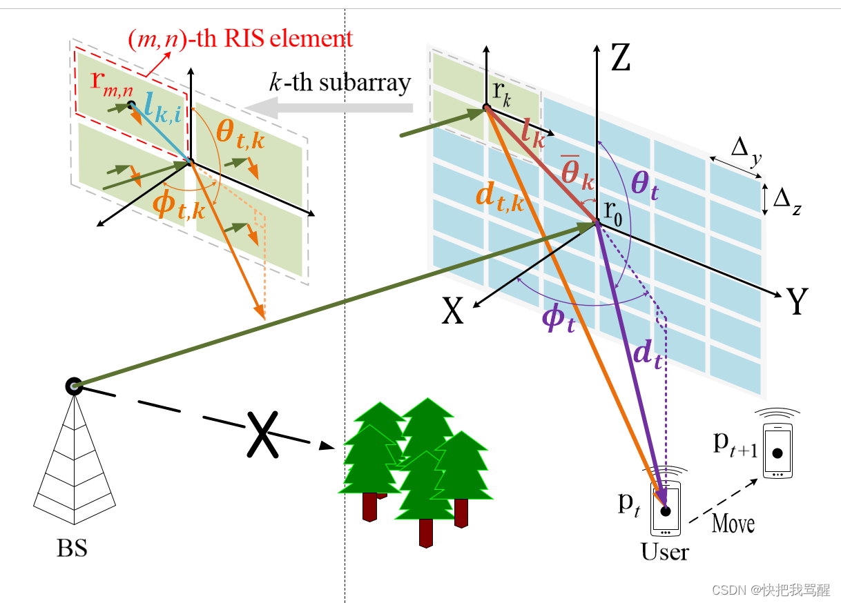
师姐论文的图，可以明显看到需要考虑阵列中每个阵元到BS（或者用户）的矢量（距离有显著不同，距离，方向）

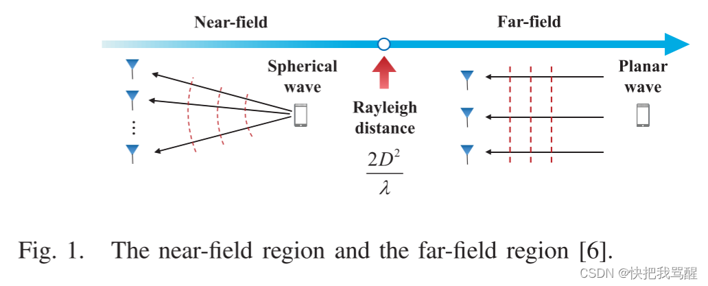
As mentioned in Section $I$ , the far-field and near-field regions are divided by the Rayleigh distance $R$ . The Rayleigh distance $R$ for the transmission array can be defined as [17]

$$R=\frac{2D^2}{\lambda }\text{\hspace{1em}(8)}$$

where $D$ is the array aperture. When the distance between this array and receiver is smaller than $R$ , the receiver locates in the near-field region of this array and the channel has to be modeled as near-field channel. Moreover, for a XL-RIS aided system, when the distance $r_{\mathrm{RA}}$ between the XL-RIS and the $\mathrm{BS}$ and the distance $r_{\mathrm{RD}}$ between the XL-RIS and the user satisfy

$$\frac{r_{\mathrm{RA}}{r}_{\mathrm{RD}}}{r_{\mathrm{RA}}+r_{\mathrm{RD}}}<R=\frac{2D^2}{\lambda }\text{\hspace{1em}(9)}$$

反射信道应建模为近场通道[17]。从（9）我们可以发现，只要任何一个BS或用户分布在XLRIS的近场区域，与该反射链路相关的通信就应该考虑近场特征来制定[17] ]。因此，对于XL-RIS辅助的无线通信，近场场景更为普遍。

由式（9）可知，瑞利距离与阵列孔径的平方成正比。对于阵元间距固定的阵列，**随着阵列孔径从RIS增加到XL-RIS，瑞利距离将呈二次方增加。因此，如图2所示，近场区域将会扩大。结果，BS和用户更有可能散布在近场区域。**例如，如果载波频率为 $10GHz$（即 $\lambda =3\times 10^{-2}m$），RIS 的阵列孔径为 $D_{RIS}=0.3$ m，则瑞利距离为 $R_{RIS}=6m$。对于阵列孔径 $D_{XL-RIS}=1.2m$ 的 XL-RIS，瑞利距离将增加至 $R_{XL-RIS}=96m$。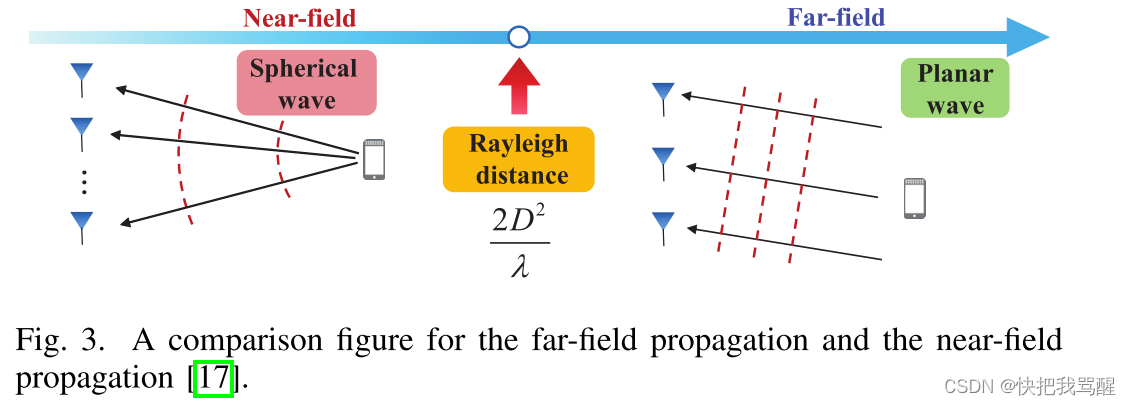

在远场场景中，在平面波前假设下对信道进行建模，基于该假设，远场导向矢量在数学上被描述为（5）。对于这种情况，物理学上更直观的解释可以如图3右侧所示，即电磁波的等相波前可以近似视为共面。相反，在图3左侧所示的近场场景中，在球面波前假设下对电磁波进行建模更加准确，而遵循平面波前假设会在近场带来严重的相位误差区[17]。

---

在近场场景下，有效反射通道 ${\overline{\mathbf{h}}}_{\mathrm{NF},k}$可以重写为[26]

$${\overline{\mathbf{h}}}_{\mathrm{NF},k}={\bar{\alpha }}_k\mathrm{diag}\left({\mathbf{b}}^T\left({\mathbf{r}}_{\mathrm{re},k}\right)\right)\mathbf{b}\left({\mathbf{r}}_{\mathrm{in}}\right),\text{\hspace{1em}(10)}$$

where ${\mathbf{r}}_{\mathrm{re},k}$ is the space coordinate vector from the XL-RIS to the $k$ th user, and ${\mathbf{r}}_{\text{in }}$ is the space coordinate vector from the BS to the XL-RIS. ${\mathbf{b}}^T\left({\mathbf{r}}_{\mathrm{re},k}\right)$ and $\mathbf{b}\left({\mathbf{r}}_{\mathrm{in}}\right)$ in (10) can be denoted as

$$\begin{array}{rl}\mathbf{b}\left({\mathbf{r}}_{\mathrm{re},k}\right)=& [e^{-j2\pi D_k^{\mathrm{re}}(1,1)},\cdots ,e^{-j2\pi D_k^{\mathrm{re}}\left(1,N_2\right)},\cdots ,\\ & {e^{-j2\pi D_k^{\mathrm{re}}\left(N_1,1\right)},\cdots ,e^{-j2\pi D_k^{\mathrm{re}}\left(N_1,N_2\right)}]}^T,\\ \mathbf{b}\left({\mathbf{r}}_{\mathrm{in}}\right)=& [e^{-j2\pi D^{\mathrm{in}}(1,1)},\cdots ,e^{-j2\pi D^{\mathrm{in}}\left(1,N_2\right)},\cdots ,\\ & {e^{-j2\pi D^{\mathrm{in}}\left(N_1,1\right)},\cdots ,e^{-j2\pi D^{\mathrm{in}}\left(N_1,N_2\right)}]}^T,\end{array}\text{\hspace{1em}(11)}$$

$\text{ where }{D}_k^{\mathrm{re}}\left(n_1,n_2\right)\text{ and }{D}^{\mathrm{in}}\left(n_1,n_2\right)\text{ denote the distance from }$ the $\left(n_1,n_2\right)$ -th element of the XL-RIS to the $k$ th user and the BS, respectively.

We can find that the main difference between the nearfield channel ${\overline{\mathbf{h}}}_{\mathrm{NF},k}$ in 10 and the far-field channel ${\overline{\mathbf{h}}}_{\mathrm{FF},k}$ in (7) is the steering vector $\mathbf{b}(\cdot )$. Specifically, the far-field steering vector $\mathbf{b}(\varphi ,\phi )$ is derived under the planar wavefront assumption, i.e., the steering vector is only related to the angles between the XL-RIS and the users (or BS). However, the steering vector $\mathbf{b}\left({\mathbf{r}}_{\mathrm{re},k}\right)$ (or $\mathbf{b}\left({\mathbf{r}}_{\mathrm{in}}\right)$ ) in the near-field is related to not only the angles but also the distances, since ${\mathbf{r}}_{\mathrm{re},k}$ (or ${\mathbf{r}}_{\text{in }})$ is a directed vector.

考虑到（7）和（10）之间的根本区别，现有的为远场波束训练设计的远场码本（例如离散傅里叶变换（DFT）码本[38]）不再适用。最近提出了分层近场码本和相应的分层近场波束训练方案[26]。然而，由于XL-RIS存在恒模约束，如果我们在多用户场景中直接使用该码本，将会带来严重的性能损失。为了解决这个问题，我们提出了一种多波束设计方法，这将在下一节中讨论。

[38] X. Wei and L. Dai, “Channel estimation for extremely large-scale
massive MIMO: Far-field, near-field, or hybrid-field?” IEEE Commun.
Lett., vol. 26, no. 1, pp. 177–181, Jan. 2022.

基于码本的beamforming设计？

提出的多波束设计方法

在本节中，我们设计了 XL-RIS 辅助无线通信的多波束设计方法来设计无源波束形成矢量。该方法由波束训练过程和多波束设计过程组成。

直观地，我们绘制图4来展示使用该方法进行波束设计的过程以及随时间的数据传输。具体地，第一过程由所有用户独立执行，以获取每个用户期望的单波束方向和期望的波束增益。然后，根据这些波束参数，在多波束设计过程中设计XL-RIS的波束形成向量。最后，该波束成形向量将用于数据传输。

step1 波束训练过程

正如第一节中提到的，通过利用波束训练，我们不需要通过信道估计[39]获得准确的CSI来设计RIS波束成形。相反，我们可以通过波束训练过程直接确定 RIS 波束成形向量。首先，BS通过RIS向用户发送训练信号。这个阶段由几个框架组成。在不同的帧期间，RIS波束成形根据预先设计的码本$\mathcal{C}$的不同码字进行配置[26]。其次，用户将测量不同帧的接收信号的功率。然后，根据最大接收功率选择所需的码字。最后，这个选择将通过上行传输反馈给BS，并且XLRIS用于数据传输的波束赋形向量将被确定为这个码字。波束训练过程可以建模为获取所需的 RIS 波束形成$\theta$满足

$$\mathbf{\theta }=\underset{{\mathbf{c}}_i\in \mathcal{C}}{\mathrm{argmax}}\left|{\overline{\mathbf{h}}}_{\mathrm{NF}}^T{\mathbf{c}}_i\right|,\text{\hspace{1em}(12)}$$

where ${\overline{\mathbf{h}}}_{\mathrm{NF}}$ is the near-field reflecting channel, and ${\mathbf{c}}_i$ is the codeword for RIS beamforming selected from $\mathcal{C}$ .

对于多用户情况，这个过程可以顺序执行，基于此我们可以获得第$k$个用户的RIS波束成形为${\theta }_{\mathbf{k}}$。然而，由于XL-RIS的恒模约束，如果我们直接叠加这些波束成形向量，将会带来严重的服务质量损失。我们的工作[26]可以支持本文中的波束训练过程。我们在下一小节中重点讨论具有挑战性的多波束设计过程，以处理恒模量约束的影响。

step2 多波束设计过程

考虑到近场信道与角度信息以及距离信息相关，近场码本网格$S$通常较大，基于此会给多波束设计带来较高的计算复杂度。请注意，与整个空间每个网格的波束增益相比，我们更关心指向 $K$ 个用户位置的波束增益。因此，在所提出的近场多波束设计过程中，仅考虑指向$K$个用户的$K$个波束的实际性能。具体来说，多波束优化问题可以表示为

$$\begin{array}{rl}{\mathcal{P}}_{NF}:\underset{\mathbf{\theta }}{\min }& l_1={\Vert \overline{\mathbf{g}}-{\mathbf{\Xi }}^H\mathbf{\theta }\Vert }_2^2\\ \text{ s.t. }& \mathrm{C}:\left|{\theta }_n\right|=1,\forall n\in \mathcal{N}\end{array}\text{\hspace{1em}(13)}$$

其中 XL-RIS 波束成形向量 $\theta$ 是要优化的变量，$\mathbf{\Xi }\in {\mathbb{C}}^{N\times K}$ 是引导(steering matrix)矩阵。 $\mathbf{\Xi }$由$K$列组成，其中第$k$列是通过波束训练过程获得的码字${\theta }_k$。$\overline{\mathbf{g}}\in {\mathbb{C}}^{K\times 1}$ 是波束增益向量，并且 $\overline{\mathbf{g}}$ 对应的元素幅度是 $K$ 个期望方向的期望波束增益。 ${\mathcal{P}}_{NF}$ 的目标函数可以重写为

Enabling More Users to Benefit from Near-Field Communications: From Linear to Circular Array

5G的大规模多输入多输出（MIMO）正在演变为超大规模天线阵列（ELAA），以提高6 G通信的频谱效率。ELAA引入了基于球面波的近场通信，其中信道容量可以显著提高单用户和多用户场景。不幸的是，广泛研究的均匀线阵（ULA）在大入射/出射角下的近场区域大大减小。因此，许多随机分布的用户可能无法受益于近场通信。在本文中，我们利用均匀圆形阵列（UCA）的旋转对称性提供均匀和扩大的近场区域在所有角度，使更多的用户受益于近场通信。具体地，利用UCA和用户之间的几何关系，开发了UCA的近场波束形成技术。基于近场波束形成的分析，我们发现，UCA是能够提供一个更大的近场区域比ULA方面的有效瑞利距离。此外，一个同心环码本的设计，以实现有效的码本波束形成在近场区域。此外，我们发现，UCA可以产生沿着相同方向的正交近场光束时，近场光束的焦点正好是其他光束的零点，这有潜力进一步提高频谱效率，在多用户通信相比ULA。仿真结果验证了理论分析的有效性和UCA的可行性，使更多的用户受益于近场通信通过拓宽近场区域。

近场MIMO综述 Near-Field MIMO Communications for 6G: Fundamentals, Challenges, Potentials, and Future Directions

入射到BS天线上的电磁波的真实相位必须基于精确的球面波模型来计算。在远场情况下，该相位通常通过基于平面波前模型的一阶泰勒展开来近似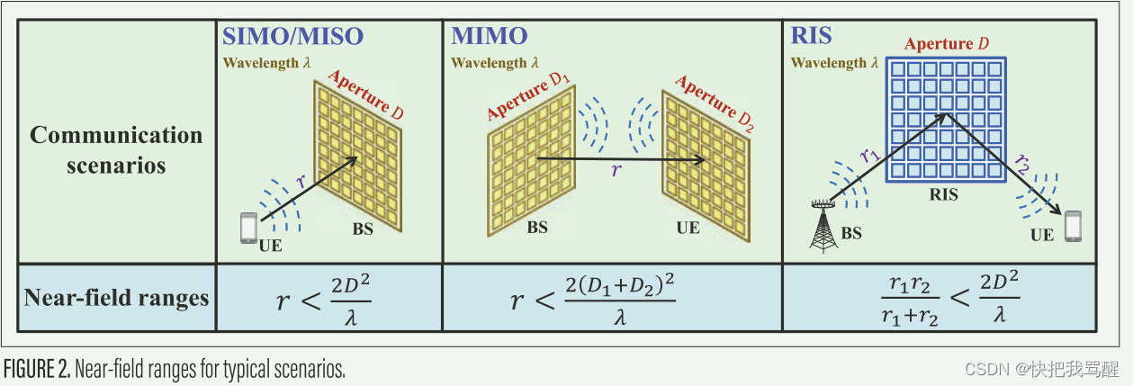
。

近场通信的挑战

近场传播给无线通信带来了一些挑战;因此，特定于远场的现有5G传输方法在近场区域中遭受严重的性能损失。本节讨论了最近开发的用于应对这些挑战的技术。

/1 近场信道估计

挑战: 为了获得ELAA的预期性能增益，需要精确的信道估计。由于信道路径的数量通常远小于天线的数量，因此具有低导频开销的信道估计方法通常设计合适的码本以将信道变换为稀疏表示。对于远场码本，码本的每个码字对应于与一个入射角相关联的平面波。理想地，每个远场路径可以仅由一个码字表示。利用该远场码本，可以获得信道的角度域表示，并且由于有限的路径，它通常是稀疏的。然后，波束训练和压缩感知（CS）的方法应用于远场信道的准确估计与低导频开销。然而，该远场平面波码本与实际的近场球面波信道不匹配。该失配指示单个近场路径应当由远场码本的多个码字联合描述。因此，近场角域信道不再稀疏，这不可避免地导致信道估计精度的降低。因此，需要仔细创建适合于近场信道的近场码本。

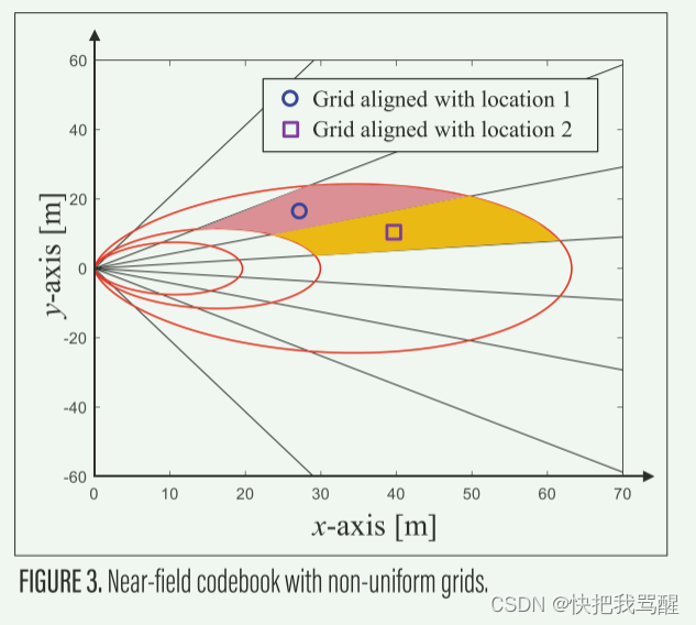
最新进展：最近的一些工作已经致力于设计利用球面波前的近场码本[5，6]。在[6]中，整个二维物理空间被均匀划分为多个网格。每个网格与近场阵列响应矢量相关联，并且所有这些矢量构成近场码本。利用该码本，提取每个近场路径的联合角度-距离信息。然后，近场信道可以估计的CS方法与低导频开销。然而，随着BS-UE距离的减小，近场传播变得占主导地位，并且距离信息逐渐变得更加关键。因此，我们可以设想的直觉，网格应该稀疏如果离ELAA较远，但密集在ELAA附近。在不考虑这种直觉的情况下，[6]中的码本难以在整个近场区域中获得令人满意的信道估计性能。为此，通过最小化近场码本中的码字之间的最大相干性，[5]中的作者在数学上证明了这种直觉（即，角度空间可以被均匀划分，而距离空间应当被非均匀划分）。如图3、距离越短，网格越密。在这种非均匀码本的帮助下，[5]中提出了极域稀疏信道表示和相应的基于CS的算法，以在近场和远场区域中实现精确的信道估计。

BS ELAA首先被划分成多个子阵列。假设UE位于每个小子阵列的远场区域中，但在ELAA的近场范围内。然后，一个TTD线插入每个子阵列和射频（RF）链之间，以实现频率相关的相移。

/1 近场波束分裂（Near Field Beam Split）

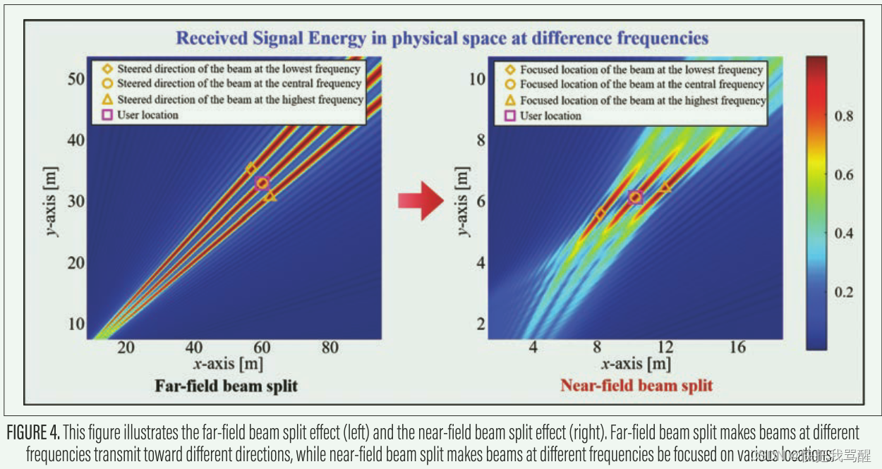
挑战：在THz宽带系统中，ELAA可能会遇到波束分裂现象，也称为波束偏斜和空间宽带效应。现有的THz波束成形架构通常采用模拟移相器（PS）[7]，其通常针对不同频率的信号调谐相同的相移。然而，EM波的实际相位是信号传播延迟和频率相关波数的乘积。结果，仅对于窄带信号，信号传播延迟可以通过相移来充分补偿。对于其他频率引入相位误差，从而引起波束分裂效应。事实上，波束分裂对远场和近场传播的影响也不同。

在远场中，波束分裂导致不同频率的波束朝向不同角度发射的事实，如图4的左侧所示。然而，对于近场光束分裂，由于球面波的分裂，光束聚焦在不同的角度和不同的距离，如图4的右侧所示。远场和近场波束分裂都严重降低了与用户位置不对准的频率分量的接收信号能量。多年来，已经提出了大量的工作来通过调谐频率相关相移与平面波阵面，通过基于真时延（TTD）的波束成形代替基于PS的波束成形来减轻远场波束分裂。不幸的是，由于平面波和球面波之间的差异，这些解决远场波束分裂的方案在近场不再工作，为太赫兹ELAA通信带来了挑战。

最新进展：最近，一些努力已经试图克服近场波束分裂效应。在[8]中，利用啁啾序列的变体来设计相移，以在牺牲最大波束聚焦增益的情况下在频率上平坦化波束聚焦增益。这种方法可以稍微减轻近场光束分裂效应，但当带宽非常大时，其频谱效率也会下降，因为波束仍然由PS产生。为此，在[9]中提出了利用基于TTD的波束成形的相位延迟聚焦（PDF）方法。为了进一步说明，BS ELAA首先被划分成多个子阵列。假设UE位于每个小子阵列的远场区域中，但在ELAA的近场范围内。然后，一个TTD线插入每个子阵列和射频（RF）链之间，以实现频率相关的相移。最后，通过插入的TTD线来补偿由球面波前引起的不同子阵列的频率相关相位变化。结果，工作频带上的波束聚焦在目标UE位置[9]。

总之，第一种解决方案[8]遵循基于PS的波束成形，其易于实现，但可实现的性能不令人满意。第二种方案[9]几乎可以消除近场分束效应，但需要实现TTD线。事实上，虽然已经在频域中证明了通过光纤部署TTD线路，但这种部署扩展到太赫兹ELAA通信是不平凡的。幸运的是，基于石墨烯的等离子体波导的最新进展提供了用于在高频下实现TTD线的低成本解决方案[7]。

幸运的是，近场波束聚焦享有能量聚焦在联合角度-距离域的能力。因此，近场SDMA可以生成具有球形波前的波束，以同时服务位于相似角度但不同距离的用户。