cc和毫升换算_如何解释你的毫升模型

Explainability in machine learning (ML) and artificial intelligence (AI) is becoming increasingly important. With the increased demand for explanations and the number of new approaches out there, it could be difficult to know where to start. In this post, we will get hands-on experience in explaining an ML model using a couple of approaches. By the end of it, you will have a good grasp of some fundamental ways in which you can explain the decisions or behavior of most machine learning models.

机器学习(ML)和人工智能(AI)的可解释性变得越来越重要。 随着对解释的需求增加以及那里出现新方法的数量，可能很难知道从哪里开始。 在本文中，我们将获得使用两种方法解释ML模型的动手经验。 到最后，您将掌握一些基本方法，可以用来解释大多数机器学习模型的决策或行为。

Types of explainability approaches

可解释性方法的类型

When it comes to explaining the models and/or their decisions, multiple approaches exist. One may want to explain the global (overall) model behavior or provide a local explanation (i.e. explain the decision of the model about each instance in the data). Some approaches are applied before the building of the model, others after the training (post-hoc). Some approaches explain the data, others the model. Some are purely visual, others not.

在解释模型和/或其决策时，存在多种方法。 可能需要解释全局 (总体)模型行为或提供局部解释(即，解释关于数据中每个实例的模型决策)。 在构建模型之前应用了一些方法，在训练之后(事后)应用了其他方法。 一些方法解释了数据，另一些方法则解释了模型。 有些纯粹是视觉的，有些则不是。

What you will need?

您需要什么？

To follow this tutorial, you will need Python 3 and some ML knowledge as I will not explain how the model I will train works. My advice is to create and work in a virtual environment because you will need to install a few packages and you may not want them to disrupt your local conda or pip setting.

要学习本教程，您将需要Python 3和一些ML知识，因为我不会解释我将训练的模型如何工作。 我的建议是在虚拟环境中创建和工作，因为您将需要安装一些软件包，并且可能不希望它们破坏您的本地conda或pip设置。

Import data and packages

导入数据和包

We will use the diabetes data set from sklearn and train a standard random forest regressor. Refer to the sklearn documentation to know more about the data (https://scikit-learn.org/stable/datasets/index.html )

我们将使用sklearn的糖尿病数据集并训练标准的随机森林回归。 请参阅sklearn文档以了解有关数据的更多信息( https://scikit-learn.org/stable/datasets/index.html )

from sklearn.datasets import load_diabetesimport pandas as pdimport matplotlib.pyplot as pltfrom sklearn.ensemble import RandomForestRegressorimport pycebox.ice as iceboxfrom sklearn.tree import DecisionTreeRegressor

Import data and train a model

导入数据并训练模型

We import the diabetes data set, assign the target variable to a vector of dependent variables y, the rest to a matrix of features X, and train a standard random forest model.

我们导入糖尿病数据集，将目标变量分配给因变量y的向量，将其余变量分配给特征X的矩阵，然后训练标准随机森林模型。

In this tutorial, I am skipping some of the typical data science steps, such as cleaning, exploring the data, and performing the conventional train/test splitting but feel free to perform those on your own.

在本教程中，我跳过了一些典型的数据科学步骤，例如清理，浏览数据以及执行常规的训练/测试拆分，但可以自行执行。

raw_data = load_diabetes()df = pd.DataFrame(np.c_[raw_data['data'], raw_data['target']],       columns= np.append(raw_data['feature_names'], ['target']))y = df.targetX = df.drop('target', axis=1)# Train a modelclf = RandomForestRegressor(random_state=42, n_estimators=50, n_jobs=-1)clf.fit(X, y)

Calculate the feature importance

计算特征重要性

We can also easily calculate and print out the feature importances after the random forest model. We see that the most important is the ‘s5’, one of the factors measuring the blood serum, followed by ‘bmi’ and ‘bp’.

我们还可以根据随机森林模型轻松计算并打印出特征重要性。 我们看到最重要的是“ s5”，它是测量血清的因素之一，其次是“ bmi”和“ bp”。

# Calculate the feature importancesfeat_importances = pd.Series(clf.feature_importances_, index=X.columns)feat_importances.sort_values(ascending=False).head()s5     0.306499bmi    0.276130bp     0.086604s6     0.074551age    0.058708dtype: float64

Visual explanations

视觉说明

The first approach I will apply is called Individual conditional expectation (ICE) plots. They are very intuitive and show you how the prediction changes as you vary the feature values. They are similar to partial dependency plots but ICE plots go one step further and reveal heterogenous effects since ICE plots display one line per instance. The below code allows you to display an ICE plot for the feature ‘bmi’ after we have trained the random forest.

我将采用的第一种方法称为个人条件期望(ICE)图。 它们非常直观，并向您展示了预测随着您更改要素值而如何变化。 它们类似于部分依存关系图，但ICE图又向前走了一步，并揭示了异质性影响，因为ICE图每个实例显示一行。 训练随机森林后，以下代码可让您显示功能'bmi'的ICE图。

# We feed in the X-matrix, the model and one feature at a time bmi_ice_df = icebox.ice(data=X, column='bmi',                    predict=clf.predict)# Plot the figurefig, ax = plt.subplots(figsize=(10, 10))plt.figure(figsize=(15, 15))icebox.ice_plot(bmi_ice_df, linewidth=.5,  plot_pdp=True,          pdp_kwargs={'c': 'red', 'linewidth': 5}, ax=ax)ax.set_ylabel('Predicted diabetes')ax.set_xlabel('BMI')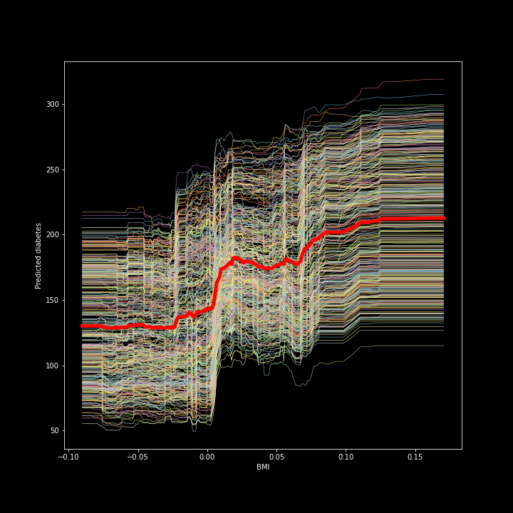

Figure 1. ICE plot for the ‘bmi’ and predicted diabetes

图1 。 ``bmi''和预测的糖尿病的ICE图

We see from the figure that there is a positive relationship between the ‘bmi’ and our target (a quantitative measure for diabetes one year after diagnosis). The thick red line in the middle is the Partial dependency plot, which shows the change in the average prediction as we vary the ‘’bmi’ feature.

从图中我们可以看出，“ bmi”与我们的目标(诊断后一年的糖尿病定量指标)之间存在正相关。 中间的粗红线是偏倚图，它显示了当我们改变“ bmi”特征时平均预测的变化。

We can also center the ICE plot, ensuring that the lines for all instances in the data start from the same point. This removes the level effects and makes the plot easier to read. We only need to change one argument in the code.

我们还可以将ICE图居中，以确保数据中所有实例的线都从同一点开始。 这样可以消除电平影响，并使图更易于阅读。 我们只需要在代码中更改一个参数即可。

icebox.ice_plot(bmi_ice_df, linewidth=.5,  plot_pdp=True,          pdp_kwargs={'c': 'blue', 'linewidth': 5}, centered=True, ax=ax1)ax1.set_ylabel('Predicted diabetes')ax1.set_xlabel('BMI')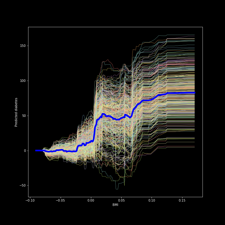

Figure 2. Centered ICE plot for the bmi and predicted diabetes

图2 。 bmi和预测糖尿病的居中ICE图

The result is a much easier to read plot!

结果是更容易阅读的情节！

Global explanations

全局说明

One popular way to explain the global behavior of a black-box model is to apply the so-called global surrogate model. The idea is that we take our black-box model and create predictions using it. Then we train a transparent model (think a shallow decision tree, linear/logistic regression) on the predictions produced by the black-box model and the original features. We need to keep track of how well the surrogate model approximates the black-box model but that is often not straightforward to determine.

解释黑盒模型的全局行为的一种流行方法是应用所谓的全局代理模型。 想法是我们采用黑盒模型并使用它创建预测。 然后，我们根据黑盒模型和原始特征产生的预测训练透明模型(认为是浅决策树，线性/逻辑回归)。 我们需要跟踪替代模型与黑盒模型的近似程度，但是通常很难直接确定。

To keep things simple, I create predictions after our random forest regressor and train a decision tree (relatively shallow one) and visualize it. That’s it! Even if we cannot easily comprehend how the hundreds of trees in the forest look (or we don’t want to retrieve them), you can build a shallow tree after it and hopefully get an idea of how the forest works.

为简单起见，我在随机森林回归器之后创建预测，并训练决策树(相对较浅的决策树)并将其可视化。 而已！ 即使我们不能轻易理解森林中数百棵树的外观(或者我们不想检索它们)，您也可以在其后建造一棵浅树，并希望对森林的工作原理有所了解。

We start with getting the predictions after the random forest and building a shallow decision tree.

我们从获得随机森林之后的预测开始，并建立一个浅层的决策树。

predictions = clf.predict(X)dt = DecisionTreeRegressor(random_state = 100, max_depth=3)dt.fit(X, predictions)Now we can plot and see how the tree looks like.fig, ax = plt.subplots(figsize=(20, 10))plot_tree(dt, feature_names=list(X.columns), precision=3,            filled=True, fontsize=12, impurity=True)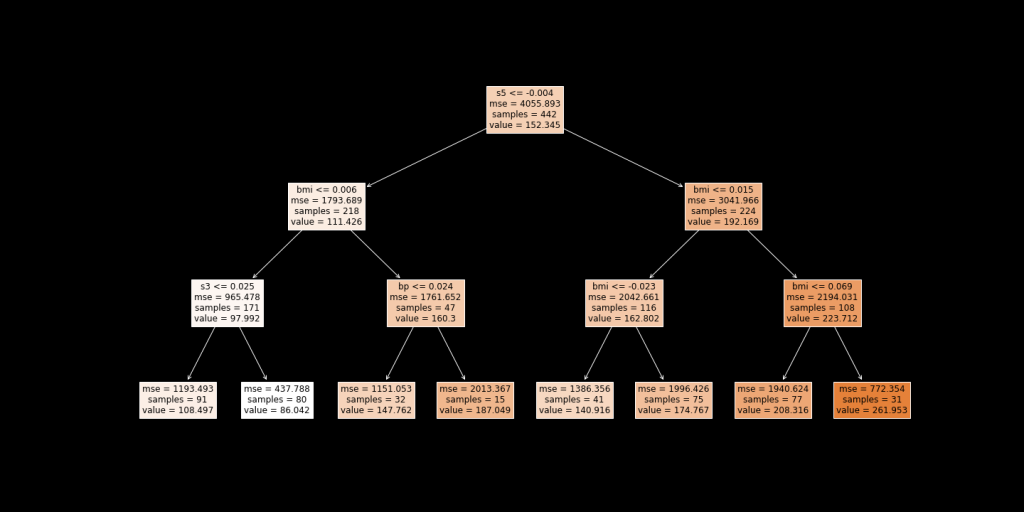

Figure 3. Surrogate model (in this case: decision tree)

图3. 代理模型(在这种情况下：决策树)

We see that the first split is at the feature ‘s5’, followed by the ‘bmi’. If you recall, these were also the two most important features picked by the random forest model.

我们看到第一个分割是在特征“ s5”处，然后是“ bmi”。 如果您还记得的话，这些也是随机森林模型选择的两个最重要的功能。

Lastly, make sure to calculate R-squared so that we can tell how good of an approximation the surrogate model is.

最后，请确保计算R平方，以便我们可以知道代理模型的近似程度。

We can do that with the code below:

我们可以使用下面的代码来做到这一点：

dt.score(X, predictions)0.6705488147404473

In this case, the R-squared is 0,67. Whether we deem this as high or low would be very context-dependent.

在这种情况下，R平方为0.67。 我们认为这是高还是低将取决于上下文。

Next steps

下一步

Now you have gained some momentum and applied explainability techniques after an ML model. You can take another dataset, or apply them to a real use case.

现在，您已经获得了一些动力，并且在ML模型之后应用了可解释性技术。 您可以获取另一个数据集，或将其应用于实际用例。

You can also join my upcoming workshop titled “Explainable ML: Application of Different Approaches’”during ODSC Europe 2020. In the workshop, we will walk through these approaches in more detail and apply other equally fascinating explainability techniques.

您也可以参加即将举行的ODSC Europe 2020主题为“ 可解释的ML：应用不同方法 ”的研讨会。在该研讨会中，我们将更详细地介绍这些方法，并应用其他同样引人入胜的解释性技术。

About the Author:

关于作者：

Violeta Misheva works as a data scientist who holds a PhD degree in applied econometrics from the Erasmus School of Economics. She is passionate about AI for good and is currently interested in fairness and explainability in machines. She enjoys sharing her data science knowledge with others, that’s why part-time she conducts workshops with students, has designed a course for the DataCamp, and regularly attends and presents at conferences and other events.

Violeta Misheva是一名数据科学家，拥有伊拉斯姆斯经济学院的应用计量经济学博士学位。 她一直对AI充满热情，目前对机器的公平性和可解释性感兴趣。 她喜欢与他人分享她的数据科学知识，这就是为什么她兼职与学生进行研讨会，为DataCamp设计课程，并定期参加会议和其他活动并进行演讲。