本文主要是介绍时间序列预测(9) — Informer源码详解与运行,希望对大家解决编程问题提供一定的参考价值,需要的开发者们随着小编来一起学习吧!
目录
1 源码解析
1.1 文件结构
1.2 mian_informer.py文件
1.3 模型训练
1.4 模型测试
1.5 模型预测
2 Informer模型
2.1 process_one_batch
2.2 Informer函数
2.3 DataEmbedding函数
2.4 ProbAttention稀疏注意力机制
2.5 Encoder编码器函数
2.6 Decoder解码器函数
3 官方数据集运行
1 源码解析
1.1 文件结构
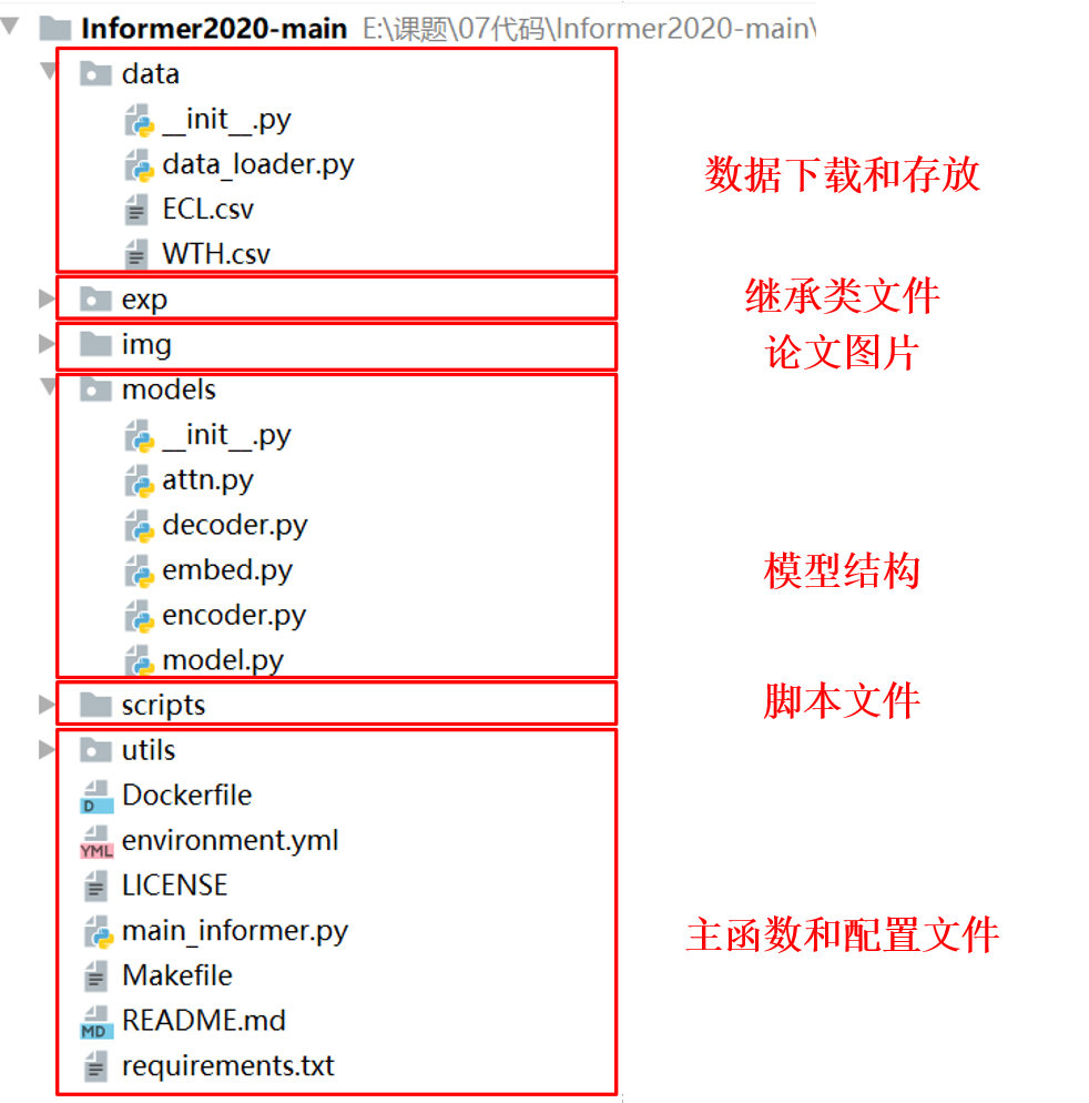
1.2 mian_informer.py文件
首先导入代码的基本函数和数据类型,在exp文件下exp_informer import中的类Exp_Informer中,定义了模型参数、get_data、model_optim、train、test、eval等函数
# 继承了exp文件下exp_informer import中的Exp_Informer
from exp.exp_informer import Exp_Informer
进一步解析模型需要的参数,参数的含义如下表格:
| 参数名称 | 参数类型 | 参数讲解 |
| model | str | 这是一个用于实验的参数设置,其中包含了三个选项: informer, informerstack, informerlight。根据实验需求,可以选择其中之一来进行实验,默认是使用informer模型。 |
| data | str | 数据,这个并不是你理解的你的数据集文件,而是你想要用官方定义的方法还是你自己的数据集进行定义数据加载器,如果是自己的数据集就输入custom |
| root_path | str | 这个才是你文件的路径,不要到具体的文件,到目录级别即可。 |
| data_path | str | 这个填写你文件的名称。 |
| features | str | 这个是特征有三个选项M,MS,S。分别是多元预测多元,多元预测单元,单元预测单元。 |
| target | str | 这个是你数据集中你想要预测那一列数据,假设我预测的是油温OT列就输入OT即可。 |
| freq | str | 时间的间隔,你数据集每一条数据之间的时间间隔。 |
| checkpoints | str | 训练出来的模型保存路径 |
| seq_len | int | 用过去的多少条数据来预测未来的数据 |
| label_len | int | 可以裂解为更高的权重占比的部分要小于seq_len |
| pred_len | int | 预测未来多少个时间点的数据 |
| enc_in | int | 你数据有多少列,要减去时间那一列,这里我是输入8列数据但是有一列是时间所以就填写7 |
| dec_in | int | 同上 |
| c_out | int | 这里有一些不同如果你的features填写的是M那么和上面就一样,如果填写的MS那么这里要输入1因为你的输出只有一列数据。 |
| d_model | int | 用于设置模型的维度,默认值为512。可以根据需要调整该参数的数值来改变模型的维度 |
| n_heads | int | 用于设置模型中的注意力头数。默认值为8,表示模型会使用8个注意力头,我建议和的输入数据的总体保持一致,列如我输入的是8列数据不用刨去时间的那一列就输入8即可。 |
| e_layers | int | 用于设置编码器的层数 |
| d_layers | int | 用于设置解码器的层数 |
| s_layers | str | 用于设置堆叠编码器的层数 |
| d_ff | int | 模型中全连接网络(FCN)的维度,默认值为2048 |
| factor | int | ProbSparse自注意力中的因子,默认值为5 |
| padding | int | 填充类型,默认值为0,这个应该大家都理解,如果不够数据就填写0. |
| distil | bool | 是否在编码器中使用蒸馏操作。使用--distil参数表示不使用蒸馏操作,默认为True也是我们的论文中比较重要的一个改进。 |
| dropout | float | 这个应该都理解不说了,丢弃的概率,防止过拟合的。 |
| attn | str | 编码器中使用的注意力类型,默认为"prob"我们论文的主要改进点,提出的注意力机制。 |
| embed | str | 时间特征的编码方式,默认为"timeF" |
| activation | str | 激活函数 |
| output_attention | bool | 是否在编码器中输出注意力,默认为False |
| do_predict | bool | 是否进行预测,这里模型中没有给添加算是一个小bug我们需要填写一个default=True在其中。 |
| mix | bool | 在生成式解码器中是否使用混合注意力,默认为True |
| cols | str | 从数据文件中选择特定的列作为输入特征,应该用不到 |
| num_workers | int | 线程windows大家最好设置成0否则会报线程错误,linux系统随便设置。 |
| itr | int | 实验运行的次数,默认为2,我们这里改成数字1. |
| train_epochs | int | 训练的次数 |
| batch_size | int | 一次往模型力输入多少条数据 |
| patience | int | 早停机制,如果损失多少个epochs没有改变就停止训练。 |
| learning_rate | float | 学习率。 |
| des | str | 实验描述,默认为"test" |
| loss | str | 损失函数,默认为"mse" |
| lradj | str | 学习率的调整方式,默认为"type1" |
| use_amp | bool | 混合精度训练, |
| inverse | bool | 我们的数据输入之前会被进行归一化处理,这里默认为False,算是一个小bug,因为输出的数据模型没有给我们转化成我们的数据,我们要改成True。 |
| use_gpu | bool | 是否使用GPU训练,根据自身来选择 |
| gpu | int | GPU的编号 |
| use_multi_gpu | bool | 是否使用多个GPU训练。 |
| devices | str | GPU的编号 |
接下来判断是否使用GPU设备进行训练
# 判断是否使用GPU设备进行训练
args.use_gpu = True if torch.cuda.is_available() and args.use_gpu else False
if args.use_gpu and args.use_multi_gpu:args.devices = args.devices.replace(' ','')device_ids = args.devices.split(',')args.device_ids = [int(id_) for id_ in device_ids]args.gpu = args.device_ids[0]
然后解析数据集的信息,字典data_parser中包含了不同数据集的信息,键值为数据集名称('ETTh1'等),对应一个包含.csv数据文件名。接着遍历字典data_parser,将数据信息存储在data_info变量中,并将相关信息存储在args中。最后将将args.s_layers中的字符串转换为整数列表。
## 解析数据集的信息 ##
# 字典data_parser中包含了不同数据集的信息,键值为数据集名称('ETTh1'等),对应一个包含.csv数据文件名
# 目标特征、M、S和MS等参数的字典
data_parser = {'ETTh1':{'data':'ETTh1.csv','T':'OT','M':[7,7,7],'S':[1,1,1],'MS':[7,7,1]},'ETTh2':{'data':'ETTh2.csv','T':'OT','M':[7,7,7],'S':[1,1,1],'MS':[7,7,1]},'ETTm1':{'data':'ETTm1.csv','T':'OT','M':[7,7,7],'S':[1,1,1],'MS':[7,7,1]},'ETTm2':{'data':'ETTm2.csv','T':'OT','M':[7,7,7],'S':[1,1,1],'MS':[7,7,1]},'WTH':{'data':'WTH.csv','T':'WetBulbCelsius','M':[12,12,12],'S':[1,1,1],'MS':[12,12,1]},'ECL':{'data':'ECL.csv','T':'MT_320','M':[321,321,321],'S':[1,1,1],'MS':[321,321,1]},'Solar':{'data':'solar_AL.csv','T':'POWER_136','M':[137,137,137],'S':[1,1,1],'MS':[137,137,1]},
}
# 遍历字典data_parser
# 将数据信息存储在data_info变量中,并将相关信息存储在args中
# data_path:数据存放路径
# target:标签,也就是需要预测的值
# enc_in, args.dec_in, args.c_out为特征
if args.data in data_parser.keys():data_info = data_parser[args.data]args.data_path = data_info['data']args.target = data_info['T']args.enc_in, args.dec_in, args.c_out = data_info[args.features]# 首先将args.s_layers中的字符串转换为整数列表
# 它首先使用replace函数去掉空格,然后使用split函数根据逗号分隔字符串,并使用列表推导式将分割后的字符串转换为整数列表。
args.s_layers = [int(s_l) for s_l in args.s_layers.replace(' ','').split(',')]
# 参数的赋值
args.detail_freq = args.freq
args.freq = args.freq[-1:]
# 打印参数信息。
print('Args in experiment:')
print(args)
最后声明Informer模型,开始训练、验证和预测,最后清楚GPU缓存。
# 声明Informer模型对象
Exp = Exp_Informer# 开始遍历循环训练args.itr次
for ii in range(args.itr):# setting record of experimentssetting = '{}_{}_ft{}_sl{}_ll{}_pl{}_dm{}_nh{}_el{}_dl{}_df{}_at{}_fc{}_eb{}_dt{}_mx{}_{}_{}'.format(args.model, args.data, args.features, args.seq_len, args.label_len, args.pred_len,args.d_model, args.n_heads, args.e_layers, args.d_layers, args.d_ff, args.attn, args.factor, args.embed, args.distil, args.mix, args.des, ii)exp = Exp(args) # set experiments# 开始训练print('>>>>>>>start training : {}>>>>>>>>>>>>>>>>>>>>>>>>>>'.format(setting))exp.train(setting)# 开始测试print('>>>>>>>testing : {}<<<<<<<<<<<<<<<<<<<<<<<<<<<<<<<<<'.format(setting))exp.test(setting)# 开始预测if args.do_predict:print('>>>>>>>predicting : {}<<<<<<<<<<<<<<<<<<<<<<<<<<<<<<<<<'.format(setting))exp.predict(setting, True)# 清空了GPU缓存,以释放内存。torch.cuda.empty_cache()
1.3 模型训练
train代码主要实现了Informer模型的训练过程,包括数据加载、模型训练、损失计算、学习率调整和提前停止训练过程。
## 训练函数 ##def train(self, setting):# 获取训练、验证、测试数据和加载器。train_data, train_loader = self._get_data(flag = 'train')vali_data, vali_loader = self._get_data(flag = 'val')test_data, test_loader = self._get_data(flag = 'test')# 创建路径用于保存训练过程中的信息path = os.path.join(self.args.checkpoints, setting)if not os.path.exists(path):os.makedirs(path)# 记录了当前的时间戳time_now = time.time()# 训练数据加载器的步数train_steps = len(train_loader)# 提前停止训练机制,如果损失多少个epochs没有改变就停止训练。early_stopping = EarlyStopping(patience=self.args.patience, verbose=True)# 获取优化器和损失函数model_optim = self._select_optimizer()criterion = self._select_criterion()# 是否使用混合精度训练,如果使用则创建了一个if self.args.use_amp:scaler = torch.cuda.amp.GradScaler()# 这行代码开始train_epochs次循环训练。for epoch in range(self.args.train_epochs):# 初始化迭代计数器和训练损失iter_count = 0train_loss = []# 将模型设置为训练模式self.model.train()# 记录每个epoch的训练时间epoch_time = time.time()# 遍历训练数据加载器中的每个批次,并进行模型训练for i, (batch_x,batch_y,batch_x_mark,batch_y_mark) in enumerate(train_loader):iter_count += 1# 梯度清零model_optim.zero_grad()# 计算模型的预测值和真实值、损失pred, true = self._process_one_batch(train_data, batch_x, batch_y, batch_x_mark, batch_y_mark)loss = criterion(pred, true)train_loss.append(loss.item())# 打印当前迭代的信息,包括迭代次数、epoch、损失值、训练速度等if (i+1) % 100==0:print("\titers: {0}, epoch: {1} | loss: {2:.7f}".format(i + 1, epoch + 1, loss.item()))speed = (time.time()-time_now)/iter_countleft_time = speed*((self.args.train_epochs - epoch)*train_steps - i)print('\tspeed: {:.4f}s/iter; left time: {:.4f}s'.format(speed, left_time))iter_count = 0time_now = time.time()# 根据是否使用混合精度训练,选择不同的梯度更新方式if self.args.use_amp:scaler.scale(loss).backward()scaler.step(model_optim)scaler.update()else:loss.backward()model_optim.step()# 计算并打印每个epoch的训练时间、平均训练损失、验证损失和测试损失print("Epoch: {} cost time: {}".format(epoch+1, time.time()-epoch_time))train_loss = np.average(train_loss)vali_loss = self.vali(vali_data, vali_loader, criterion)test_loss = self.vali(test_data, test_loader, criterion)print("Epoch: {0}, Steps: {1} | Train Loss: {2:.7f} Vali Loss: {3:.7f} Test Loss: {4:.7f}".format(epoch + 1, train_steps, train_loss, vali_loss, test_loss))early_stopping(vali_loss, self.model, path)if early_stopping.early_stop:print("Early stopping")break# 根据当前epoch的情况,调整学习率adjust_learning_rate(model_optim, epoch+1, self.args)# 最后保存最佳模型的参数,并返回该模型best_model_path = path+'/'+'checkpoint.pth'self.model.load_state_dict(torch.load(best_model_path))return self.model1.4 模型测试
test函数主要实现了Informer模型的测试过程,包括测试数据加载、模型测试、损失计算、保存测试结果的过程。
## 测试函数 ##def test(self, setting):# 获取测试数据和测试数据加载器test_data, test_loader = self._get_data(flag='test')# 将模型设置为验证模式self.model.eval()# 初始化,存储模型的预测值和真实值preds = []trues = []# 遍历测试数据加载器中的每个批次for i, (batch_x,batch_y,batch_x_mark,batch_y_mark) in enumerate(test_loader):# 对每个批次的数据进行预测,并将预测值和真实值存储到preds和trues列表中pred, true = self._process_one_batch(test_data, batch_x, batch_y, batch_x_mark, batch_y_mark)preds.append(pred.detach().cpu().numpy())trues.append(true.detach().cpu().numpy())# 将列表转换为NumPy数组preds = np.array(preds)trues = np.array(trues)# 这两行代码对预测值和真实值进行形状调整print('test shape:', preds.shape, trues.shape)preds = preds.reshape(-1, preds.shape[-2], preds.shape[-1])trues = trues.reshape(-1, trues.shape[-2], trues.shape[-1])print('test shape:', preds.shape, trues.shape)# 保存测试结果folder_path = './results/' + setting +'/'if not os.path.exists(folder_path):os.makedirs(folder_path)# 计算并打印误差mae, mse, rmse, mape, mspe = metric(preds, trues)print('mse:{}, mae:{}'.format(mse, mae))# 分别将评估指标、预测值和真实值保存为NumPy数组文件np.save(folder_path+'metrics.npy', np.array([mae, mse, rmse, mape, mspe]))np.save(folder_path+'pred.npy', preds)np.save(folder_path+'true.npy', trues)return1.5 模型预测
predict函数利用Informer模型的最佳训练参数进行预测,包括预测数据加载、模型预测、保存预测结果的过程。
## 预测函数 ##def predict(self, setting, load=False):# 获取预测数据和预测数据加载器pred_data, pred_loader = self._get_data(flag='pred')# 加载了最佳模型的参数if load:path = os.path.join(self.args.checkpoints, setting)best_model_path = path+'/'+'checkpoint.pth'self.model.load_state_dict(torch.load(best_model_path))# 将模型设置为评估模式self.model.eval()# 初始化,存储模型的预测值preds = []# 遍历预测数据加载器中的每个批次for i, (batch_x,batch_y,batch_x_mark,batch_y_mark) in enumerate(pred_loader):# 每个批次的数据进行预测,并将预测值存储到preds列表中pred, true = self._process_one_batch(pred_data, batch_x, batch_y, batch_x_mark, batch_y_mark)preds.append(pred.detach().cpu().numpy())# 将列表转换为NumPy数组preds = np.array(preds)preds = preds.reshape(-1, preds.shape[-2], preds.shape[-1])# 保存预测结果folder_path = './results/' + setting +'/'if not os.path.exists(folder_path):os.makedirs(folder_path)np.save(folder_path+'real_prediction.npy', preds)return2 Informer模型
2.1 process_one_batch
前面介绍了训练、测试和预测的的流程,那么每一批次是数据是如何利用Informer模型进行训练的呢?首先看一下每一个批次的训练函数process_one_batch,包括数据加载、数据处理、模型训练、保存预测结果的过程。
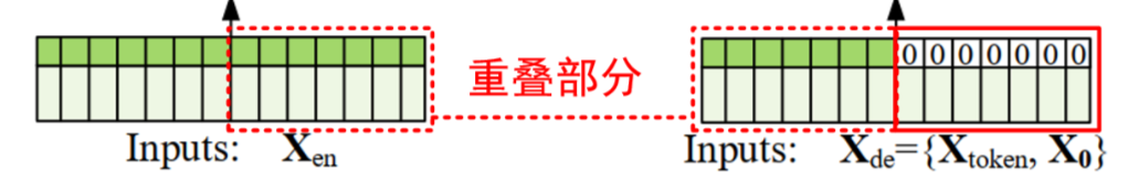
## 每一批次数据训练过程 ##def _process_one_batch(self, dataset_object, batch_x, batch_y, batch_x_mark, batch_y_mark):# 将输入数据转换为浮点型,并移到GPU设备上batch_x = batch_x.float().to(self.device)batch_y = batch_y.float()batch_x_mark = batch_x_mark.float().to(self.device)batch_y_mark = batch_y_mark.float().to(self.device)# decoder解码器输入if self.args.padding==0:# padding=0,创建一个全零的张量作为解码器输入dec_inp = torch.zeros([batch_y.shape[0], self.args.pred_len, batch_y.shape[-1]]).float()elif self.args.padding==1:# padding=1,创建一个全1的张量作为解码器输入dec_inp = torch.ones([batch_y.shape[0], self.args.pred_len, batch_y.shape[-1]]).float()# 将目标数据的一部分与解码器输入拼接在一起,就是论文结构图 X_de={X_token,X_0}dec_inp = torch.cat([batch_y[:,:self.args.label_len,:], dec_inp], dim=1).float().to(self.device)# encoder - decoder# 是否启用了混合精度训练if self.args.use_amp:with torch.cuda.amp.autocast():# 根据是否在编码器中输出注意力,进行不同的模型训练if self.args.output_attention:outputs = self.model(batch_x, batch_x_mark, dec_inp, batch_y_mark)[0]else:outputs = self.model(batch_x, batch_x_mark, dec_inp, batch_y_mark)else:if self.args.output_attention:outputs = self.model(batch_x, batch_x_mark, dec_inp, batch_y_mark)[0]else:outputs = self.model(batch_x, batch_x_mark, dec_inp, batch_y_mark)# 我们的数据输入之前会被进行归一化处理,这里对预测数据进行还原if self.args.inverse:outputs = dataset_object.inverse_transform(outputs)# 这个features有三个选项M,MS,S。分别是多元预测多元,多元预测单元,单元预测单元# 根据预测方式调整输出数据f_dim = -1 if self.args.features=='MS' else 0batch_y = batch_y[:,-self.args.pred_len:,f_dim:].to(self.device)return outputs, batch_y
2.2 Informer函数
Informer模型主函数进行Encoding -> Attention -> Encoder -> Decoder - > Linear过程,对应论文的流程图。
## Informer模型主函数 ##
class Informer(nn.Module):def __init__(self, enc_in, dec_in, c_out, seq_len, label_len, out_len, factor=5, d_model=512, n_heads=8, e_layers=3, d_layers=2, d_ff=512, dropout=0.0, attn='prob', embed='fixed', freq='h', activation='gelu', output_attention = False, distil=True, mix=True,device=torch.device('cuda:0')):super(Informer, self).__init__()self.pred_len = out_lenself.attn = attnself.output_attention = output_attention# Encodingself.enc_embedding = DataEmbedding(enc_in, d_model, embed, freq, dropout)self.dec_embedding = DataEmbedding(dec_in, d_model, embed, freq, dropout)# AttentionAttn = ProbAttention if attn=='prob' else FullAttention# Encoderself.encoder = Encoder([EncoderLayer(AttentionLayer(Attn(False, factor, attention_dropout=dropout, output_attention=output_attention), d_model, n_heads, mix=False),d_model,d_ff,dropout=dropout,activation=activation) for l in range(e_layers)],[ConvLayer(d_model) for l in range(e_layers-1)] if distil else None,norm_layer=torch.nn.LayerNorm(d_model))# Decoderself.decoder = Decoder([DecoderLayer(AttentionLayer(Attn(True, factor, attention_dropout=dropout, output_attention=False), d_model, n_heads, mix=mix),AttentionLayer(FullAttention(False, factor, attention_dropout=dropout, output_attention=False), d_model, n_heads, mix=False),d_model,d_ff,dropout=dropout,activation=activation,)for l in range(d_layers)],norm_layer=torch.nn.LayerNorm(d_model))# self.end_conv1 = nn.Conv1d(in_channels=label_len+out_len, out_channels=out_len, kernel_size=1, bias=True)# self.end_conv2 = nn.Conv1d(in_channels=d_model, out_channels=c_out, kernel_size=1, bias=True)self.projection = nn.Linear(d_model, c_out, bias=True)def forward(self, x_enc, x_mark_enc, x_dec, x_mark_dec, enc_self_mask=None, dec_self_mask=None, dec_enc_mask=None):enc_out = self.enc_embedding(x_enc, x_mark_enc)enc_out, attns = self.encoder(enc_out, attn_mask=enc_self_mask)dec_out = self.dec_embedding(x_dec, x_mark_dec)dec_out = self.decoder(dec_out, enc_out, x_mask=dec_self_mask, cross_mask=dec_enc_mask)dec_out = self.projection(dec_out)# dec_out = self.end_conv1(dec_out)# dec_out = self.end_conv2(dec_out.transpose(2,1)).transpose(1,2)if self.output_attention:return dec_out[:,-self.pred_len:,:], attnselse:return dec_out[:,-self.pred_len:,:] # [B, L, D]
2.3 DataEmbedding函数
一般Transformer框架的第一层都是embedding,把各种特征信息融合在一起,作者从3个角度进行特征融合,并执行两步DataEmbedding操作,对应论文原理图中有两部分输入 X_en 和 X_de:
# 对应论文原理图中有两部分输入 X_en 和 X_de
self.enc_embedding = DataEmbedding(enc_in, d_model, embed, freq, dropout)
self.dec_embedding = DataEmbedding(dec_in, d_model, embed, freq, dropout)
DataEmbedding操作过程如下:
class DataEmbedding(nn.Module):def __init__(self, c_in, d_model, embed_type='fixed', freq='h', dropout=0.1):super(DataEmbedding, self).__init__()self.value_embedding = TokenEmbedding(c_in=c_in, d_model=d_model)self.position_embedding = PositionalEmbedding(d_model=d_model)self.temporal_embedding = TemporalEmbedding(d_model=d_model, embed_type=embed_type,freq=freq) if embed_type != 'timeF' else TimeFeatureEmbedding(d_model=d_model, embed_type=embed_type, freq=freq)self.dropout = nn.Dropout(p=dropout)def forward(self, x, x_mark):x = self.value_embedding(x) + self.temporal_embedding(x_mark) + self.position_embedding(x)return self.dropout(x)- TokenEmbedding:用来将输入的token序列转换为向量表示,这里使用了一个一维卷积层来进行处理。
- PositionalEmbedding:用来对输入序列的位置信息进行编码,这里使用了sin和cos函数来生成位置编码。
- TemporalEmbedding:用来对输入序列的时间信息进行编码,包括分钟、小时、星期几、日期和月份等。根据不同的时间频率,选择不同的Embedding方式来进行编码。
## 将输入的token序列转换为向量表示 ##
# 这里使用了一个一维卷积层来进行处理
class TokenEmbedding(nn.Module):# c_in:输入的特征维度# d_model:嵌入后的维度def __init__(self, c_in, d_model):super(TokenEmbedding, self).__init__()# 根据PyTorch的版本选择不同的padding值padding = 1 if torch.__version__ >= '1.5.0' else 2# 将输入的token序列进行卷积操作self.tokenConv = nn.Conv1d(in_channels=c_in, out_channels=d_model,kernel_size=3, padding=padding, padding_mode='circular', bias=False)for m in self.modules():if isinstance(m, nn.Conv1d):nn.init.kaiming_normal_(m.weight, mode='fan_in', nonlinearity='leaky_relu')# 执行前向传播操作def forward(self, x):x = self.tokenConv(x.permute(0, 2, 1)).transpose(1, 2)return x
## 对输入序列的位置信息进行编码 ##
# 这里使用了sin和cos函数来生成位置编码
class PositionalEmbedding(nn.Module):def __init__(self, d_model, max_len=5000):super(PositionalEmbedding, self).__init__()# 创建了一个大小为(max_len, d_model)的全零张量pe = torch.zeros(max_len, d_model).float()# 不需要梯度更新pe.require_grad = False# 创建了一个长度为max_len的位置张量position,并将其转换为浮点型张量,并在其维度1上增加了一个维度。position = torch.arange(0, max_len).float().unsqueeze(1)# 计算得到一个长度为d_model的张量div_term = (torch.arange(0, d_model, 2).float() * -(math.log(10000.0) / d_model)).exp()# 计算了正弦和余弦位置编码# 并将结果分别赋值给pe张量的偶数索引和奇数索引位置。pe[:, 0::2] = torch.sin(position * div_term)pe[:, 1::2] = torch.cos(position * div_term)# 将pe张量增加一个维度pe = pe.unsqueeze(0)# 将位置编码pe作为模型的缓冲区self.register_buffer('pe', pe)# 执行前向传播def forward(self, x):return self.pe[:, :x.size(1)]## 时间嵌入部分 ##
class TemporalEmbedding(nn.Module):def __init__(self, d_model, embed_type='fixed', freq='h'):super(TemporalEmbedding, self).__init__()# 分别表示分钟、小时、星期、日期和月份的维度大小minute_size = 4hour_size = 24weekday_size = 7day_size = 32month_size = 13# embed_type参数选择使用固定嵌入(FixedEmbedding)还是普通嵌入(nn.Embedding)Embed = FixedEmbedding if embed_type == 'fixed' else nn.Embedding# 是否初始化了分钟嵌入向量,并进行时间嵌入操作if freq == 't':self.minute_embed = Embed(minute_size, d_model)self.hour_embed = Embed(hour_size, d_model)self.weekday_embed = Embed(weekday_size, d_model)self.day_embed = Embed(day_size, d_model)self.month_embed = Embed(month_size, d_model)2.4 ProbAttention稀疏注意力机制
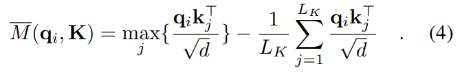
主要思想是在计算每个quey稀疏性得分时,只需采样出的部分和key计算就可以了。就是找到这些重要的/稀疏的query,从而只计算这些queryl的attention值,来优化计算效率。
## 概率稀疏注意力机制 ##
class ProbAttention(nn.Module):# mask_flag(是否使用掩码)# factor(用于计算稀疏性的因子)# scale(缩放因子)# attention_dropout(注意力机制的dropout率)# output_attention(是否输出注意力权重)def __init__(self, mask_flag=True, factor=5, scale=None, attention_dropout=0.1, output_attention=False):super(ProbAttention, self).__init__()self.factor = factorself.scale = scaleself.mask_flag = mask_flagself.output_attention = output_attentionself.dropout = nn.Dropout(attention_dropout)# prob_QK方法用于计算概率稀疏注意力机制中的Q_K矩阵,其中包括了对Q和K的采样、稀疏性计算和计算Q_K矩阵def _prob_QK(self, Q, K, sample_k, n_top): # n_top: c*ln(L_q)# Q [B, H, L, D]# 获取张量K和Q的形状信息# 分别表示批量大小、头数、K序列长度和嵌入维度B, H, L_K, E = K.shape_, _, L_Q, _ = Q.shape## calculate the sampled Q_K,对应论文中的公式(4)### 张量K沿着第三个维度进行扩展,以便与Q相乘K_expand = K.unsqueeze(-3).expand(B, H, L_Q, L_K, E)# 生成一个(L_Q, sample_k)大小的随机整数张量,用于在K中进行采样index_sample = torch.randint(L_K, (L_Q, sample_k)) # real U = U_part(factor*ln(L_k))*L_q# 获取采样的K张量K_sample = K_expand[:, :, torch.arange(L_Q).unsqueeze(1), index_sample, :]# 计算稀疏性测量值MQ_K_sample = torch.matmul(Q.unsqueeze(-2), K_sample.transpose(-2, -1)).squeeze(-2)# find the Top_k query with sparisty measurement# 计算稀疏性测量值M,包括对Q_K采样进行最大值计算和求和计算,对应论文中的公式(4)M = Q_K_sample.max(-1)[0] - torch.div(Q_K_sample.sum(-1), L_K)# 找到稀疏性最高的查询项,即M中top-k的索引M_top = M.topk(n_top, sorted=False)[1]# use the reduced Q to calculate Q_K# 计算最终的Q_K矩阵,即使用减少的Q和K进行点积计算Q_reduce = Q[torch.arange(B)[:, None, None],torch.arange(H)[None, :, None],M_top, :] # factor*ln(L_q)Q_K = torch.matmul(Q_reduce, K.transpose(-2, -1)) # factor*ln(L_q)*L_kreturn Q_K, M_topdef _get_initial_context(self, V, L_Q):# 张量V的形状信息B, H, L_V, D = V.shape# 判断是否使用掩码if not self.mask_flag:# 如果不使用掩码,计算V在倒数第二维上的均值,得到V的总和# V_sum = V.sum(dim=-2)V_sum = V.mean(dim=-2)# 将V_sum扩展为与查询序列相同长度的向量contex = V_sum.unsqueeze(-2).expand(B, H, L_Q, V_sum.shape[-1]).clone()else: # use mask# 如果使用掩码,需要L_Q == L_V,然后对V进行累积求和assert(L_Q == L_V) # requires that L_Q == L_V, i.e. for self-attention onlycontex = V.cumsum(dim=-2)return contex## 更新def _update_context(self, context_in, V, scores, index, L_Q, attn_mask):B, H, L_V, D = V.shape# 如果使用掩码,更新注意力掩码if self.mask_flag:attn_mask = ProbMask(B, H, L_Q, index, scores, device=V.device)scores.masked_fill_(attn_mask.mask, -np.inf)# 对注意力分数进行softmax操作,得到注意力权重attn = torch.softmax(scores, dim=-1) # nn.Softmax(dim=-1)(scores)# 使用注意力权重对输入张量V进行加权求和context_in[torch.arange(B)[:, None, None],torch.arange(H)[None, :, None],index, :] = torch.matmul(attn, V).type_as(context_in)# 是否需要输出注意力权重if self.output_attention:attns = (torch.ones([B, H, L_V, L_V])/L_V).type_as(attn).to(attn.device)attns[torch.arange(B)[:, None, None], torch.arange(H)[None, :, None], index, :] = attnreturn (context_in, attns)else:return (context_in, None)## 前项传播操作def forward(self, queries, keys, values, attn_mask):B, L_Q, H, D = queries.shape_, L_K, _, _ = keys.shapequeries = queries.transpose(2,1)keys = keys.transpose(2,1)values = values.transpose(2,1)U_part = self.factor * np.ceil(np.log(L_K)).astype('int').item() # c*ln(L_k)u = self.factor * np.ceil(np.log(L_Q)).astype('int').item() # c*ln(L_q) U_part = U_part if U_part<L_K else L_Ku = u if u<L_Q else L_Qscores_top, index = self._prob_QK(queries, keys, sample_k=U_part, n_top=u) # add scale factorscale = self.scale or 1./sqrt(D)if scale is not None:scores_top = scores_top * scale# get the contextcontext = self._get_initial_context(values, L_Q)# update the context with selected top_k queriescontext, attn = self._update_context(context, values, scores_top, index, L_Q, attn_mask)return context.transpose(2,1).contiguous(), attn
2.5 Encoder编码器函数
编码器旨在提取长顺序输入的稳健长程依赖性,Encoder编码器的实现
![]()
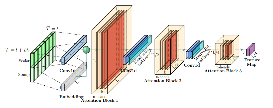
## 编码器Encoder ##
class Encoder(nn.Module):def __init__(self, attn_layers, conv_layers=None, norm_layer=None):super(Encoder, self).__init__()# 将输入的注意力层、卷积层列表转换为nn.ModuleList类self.attn_layers = nn.ModuleList(attn_layers)self.conv_layers = nn.ModuleList(conv_layers) if conv_layers is not None else Noneself.norm = norm_layerdef forward(self, x, attn_mask=None):# x [B, L, D]# 保存每个注意力层的注意力权重attns = []# 判断是否存在卷积层# 遍历注意力层和卷积层,进行前向传播计算if self.conv_layers is not None:for attn_layer, conv_layer in zip(self.attn_layers, self.conv_layers):x, attn = attn_layer(x, attn_mask=attn_mask)x = conv_layer(x)attns.append(attn)x, attn = self.attn_layers[-1](x, attn_mask=attn_mask)attns.append(attn)else:for attn_layer in self.attn_layers:x, attn = attn_layer(x, attn_mask=attn_mask)attns.append(attn)if self.norm is not None:x = self.norm(x)return x, attns
其中编码器层的实现如下:
## 编码器层 ##
class EncoderLayer(nn.Module):def __init__(self, attention, d_model, d_ff=None, dropout=0.1, activation="relu"):super(EncoderLayer, self).__init__()#  如果未提供全连接层维度d_ff,则将其设置为4*d_modeld_ff = d_ff or 4*d_modelself.attention = attention# 定义卷积、归一化、Dropout、激活函数类型选择self.conv1 = nn.Conv1d(in_channels=d_model, out_channels=d_ff, kernel_size=1)self.conv2 = nn.Conv1d(in_channels=d_ff, out_channels=d_model, kernel_size=1)self.norm1 = nn.LayerNorm(d_model)self.norm2 = nn.LayerNorm(d_model)self.dropout = nn.Dropout(dropout)self.activation = F.relu if activation == "relu" else F.gelu#  定义了EncoderLayer类的前向传播方法def forward(self, x, attn_mask=None):# x [B, L, D]# x = x + self.dropout(self.attention(#     x, x, x,#     attn_mask = attn_mask# ))new_x, attn = self.attention(x, x, x,attn_mask = attn_mask)x = x + self.dropout(new_x)y = x = self.norm1(x)y = self.dropout(self.activation(self.conv1(y.transpose(-1,1))))y = self.dropout(self.conv2(y).transpose(-1,1))return self.norm2(x+y), attn
2.6 Decoder解码器函数
提出了生成式的decoder机制,在预测序列(也包括inferencel阶段)时一步得到结果,而不是step-by-step,直接将预测时间复杂度降低。
## 编码器Encoder ##
class Encoder(nn.Module):def __init__(self, attn_layers, conv_layers=None, norm_layer=None):super(Encoder, self).__init__()# 将输入的注意力层、卷积层列表转换为nn.ModuleList类self.attn_layers = nn.ModuleList(attn_layers)self.conv_layers = nn.ModuleList(conv_layers) if conv_layers is not None else Noneself.norm = norm_layerdef forward(self, x, attn_mask=None):# x [B, L, D]# 保存每个注意力层的注意力权重attns = []# 判断是否存在卷积层# 遍历注意力层和卷积层,进行前向传播计算if self.conv_layers is not None:for attn_layer, conv_layer in zip(self.attn_layers, self.conv_layers):x, attn = attn_layer(x, attn_mask=attn_mask)x = conv_layer(x)attns.append(attn)x, attn = self.attn_layers[-1](x, attn_mask=attn_mask)attns.append(attn)else:for attn_layer in self.attn_layers:x, attn = attn_layer(x, attn_mask=attn_mask)attns.append(attn)if self.norm is not None:x = self.norm(x)return x, attns
其中解码器层的实现如下:
## 编码器层 ##
class DecoderLayer(nn.Module):def __init__(self, self_attention, cross_attention, d_model, d_ff=None,dropout=0.1, activation="relu"):super(DecoderLayer, self).__init__()#  如果未提供全连接层维度d_ff,则将其设置为4*d_modeld_ff = d_ff or 4*d_model# 定义自注意、交叉注意力、卷积、归一化、Dropout、激活函数类型选择self.self_attention = self_attentionself.cross_attention = cross_attentionself.conv1 = nn.Conv1d(in_channels=d_model, out_channels=d_ff, kernel_size=1)self.conv2 = nn.Conv1d(in_channels=d_ff, out_channels=d_model, kernel_size=1)self.norm1 = nn.LayerNorm(d_model)self.norm2 = nn.LayerNorm(d_model)self.norm3 = nn.LayerNorm(d_model)self.dropout = nn.Dropout(dropout)self.activation = F.relu if activation == "relu" else F.gelu#  定义了DecoderLayer的前向传播方法def forward(self, x, cross, x_mask=None, cross_mask=None):x = x + self.dropout(self.self_attention(x, x, x,attn_mask=x_mask)[0])x = self.norm1(x)x = x + self.dropout(self.cross_attention(x, cross, cross,attn_mask=cross_mask)[0])y = x = self.norm2(x)y = self.dropout(self.activation(self.conv1(y.transpose(-1,1))))y = self.dropout(self.conv2(y).transpose(-1,1))return self.norm3(x+y)
3 官方数据集运行
其中定义了许多参数,在其中存在一些bug有如下的->

这个bug是因为头两行参数的,中的required=True导致的,我们将其删除掉即可,改为如下:
parser.add_argument('--model', type=str, default='informer',help='model of experiment, options: [informer, informerstack, informerlight(TBD)]')
parser.add_argument('--data', type=str, default='ETTh1', help='data')
最后写如下的脚本文件可视化预测结果:
import numpy as np
import pandas as pd
import matplotlib.pyplot as plt# 指定.npy文件路径
file_path1 = "results/informer_ETTh1_ftM_sl96_ll48_pl24_dm512_nh8_el2_dl1_df2048_atprob_fc5_ebtimeF_dtTrue_mxTrue_test_0/true.npy"
file_path2 = "results/informer_ETTh1_ftM_sl96_ll48_pl24_dm512_nh8_el2_dl1_df2048_atprob_fc5_ebtimeF_dtTrue_mxTrue_test_1/pred.npy"# 使用NumPy加载.npy文件
true_value = []
pred_value = []
data1 = np.load(file_path1)
data2 = np.load(file_path2)
print(data2)
for i in range(24):true_value.append(data2[0][i][6])pred_value.append(data1[0][i][6])# 打印内容
print(true_value)
print(pred_value)#保存数据
df = pd.DataFrame({'real': true_value, 'pred': pred_value})
df.to_csv('results.csv', index=False)   #绘制图形
fig = plt.figure(figsize=( 16, 8))
plt.plot(df['real'], marker='o', markersize=8)
plt.plot(df['pred'], marker='o', markersize=8)
plt.tick_params(labelsize = 28)
plt.legend(['real','pred'],fontsize=28)
plt.show()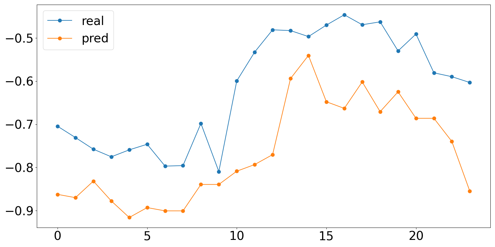
这篇关于时间序列预测(9) — Informer源码详解与运行的文章就介绍到这儿,希望我们推荐的文章对编程师们有所帮助!


