搭建PyTorch神经网络进行气温预测

前言

学习用Pytorch搭建一个两层的神经网络，用来进行气温预测。本次一共用了两种方法，一种手动构建，另一种运用Pytorch中的nn模块进行构建。

一、处理数据

1.数据读取

import pandas as pd
import matplotlib.pyplot as plt
%matplotlib inline
features = pd.read_csv('temps.csv')

读取到的数据如图所示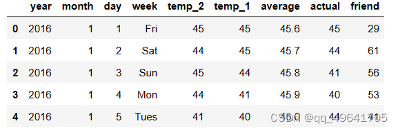
其中

• year,month,day,week分别表示具体的时间
• temp_2：前天的最高温度值
• temp_1：昨天的最高温度值
• average：在历史中，每年的这一天的平均最高温度值
• actual：真实值（标签值）
• friend：可能是朋友的猜测值

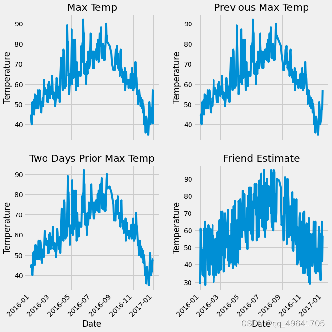
2.数据可视化（画图）

首先将数据转换为datatime格式，以便进行作图

# 处理时间数据
import datetime# 分别得到年、月、日
years =features['year']
months = features['month']
days = features['day']# datatime格式
dates = [str(int(year)) + '-' + str(int(month)) + '-' + str(int(day)) for year, month, day in zip(years, months, days)]
dates = [datetime.datetime.strptime(date, '%Y-%m-%d') for date in dates]

格式转换后进行作图

# 指定画布风格
plt.style.use('fivethirtyeight')# 设置布局 画出一个2行2列，10 × 10 的子图
fig, ((ax1, ax2),(ax3, ax4)) = plt.subplots(nrows = 2, ncols = 2, figsize = (10, 10))
fig.autofmt_xdate(rotation = 45) # x轴字体倾斜度#标签值（实际值）
ax1.plot(dates, features['actual'])
ax1.set_xlabel('');ax1.set_ylabel('Temperature');ax1.set_title('Max Temp')#昨天
ax2.plot(dates, features['temp_1'])
ax2.set_xlabel('');ax2.set_ylabel('Temperature');ax2.set_title('Previous Max Temp')#前天
ax3.plot(dates, features['temp_2'])
ax3.set_xlabel('Date');ax3.set_ylabel('Temperature');ax3.set_title('Two Days Prior Max Temp')#friend
ax4.plot(dates, features['friend'])
ax4.set_xlabel('Date');ax4.set_ylabel('Temperature');ax4.set_title('Friend Estimate')
# 自动调节子图参数，设置图像边界和子图之间的额外边距
plt.tight_layout(pad = 2) 

结果如图所示

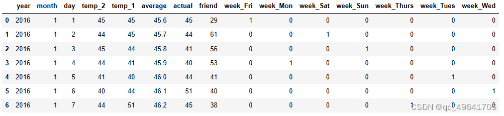
3.数据编码

由于week中是用字符串进行表示的，因此将其进行编码（采用独热编码）

# 独热编码
features = pd.get_dummies(features)

部分编码展示

4.设置标签及数据归一化

设置标签

# 标签
labels = np.array(features['actual'])# 在特征中去掉标签
features = features.drop('actual', axis = 1)#保存表头
feature_list = list(features.columns)#转换成数组格式
features = np.array(features)

数据归一化（归一化后，网络训练效果会更好）

from sklearn import preprocessing
input_features = preprocessing.StandardScaler().fit_transform(features) # 数据标准化

二、构建网络模型

1.手动构建

转换数据为tensor格式

x = torch.tensor(input_features, dtype = float)
y = torch.tensor(labels, dtype = float)

参数初始化

其中中间因此层设置128个神经元，学习率设置为0.001

weights = torch.randn((14,128), dtype = float, requires_grad = True)
biases = torch.randn(128, dtype = float, requires_grad = True)
weights2 = torch.randn((128,1), dtype = float, requires_grad = True)
biases2 = torch.randn(1, dtype = float, requires_grad = True)learning_rate = 0.001
losses = []

训练网络

其中损失的计算是计算平方值

for i in range(2000):# 计算隐层hidden = x.mm(weights) + biases# 加入激活层hidden = torch.relu(hidden)# 预测结果predictions = hidden.mm(weights2) + biases2# 计算损失loss = torch.mean((predictions - y)**2)losses.append(loss.data.numpy())# 打印损失值if i % 100 == 0:print('loss:', loss)# 反向传播计算loss.backward()#更新参数weights.data.add_(- learning_rate * weights.grad.data)biases.data.add_(- learning_rate * biases.grad.data)weights2.data.add_(- learning_rate * weights2.grad.data)biases2.data.add_(- learning_rate * biases2.grad.data)# 清空梯度weights.grad.data.zero_()biases.grad.data.zero_()weights2.grad.data.zero_()biases2.grad.data.zero_()

结果

loss: tensor(5353.6918, dtype=torch.float64, grad_fn=<MeanBackward0>)
loss: tensor(155.1765, dtype=torch.float64, grad_fn=<MeanBackward0>)
loss: tensor(147.2493, dtype=torch.float64, grad_fn=<MeanBackward0>)
loss: tensor(144.3641, dtype=torch.float64, grad_fn=<MeanBackward0>)
loss: tensor(142.8384, dtype=torch.float64, grad_fn=<MeanBackward0>)
loss: tensor(141.9417, dtype=torch.float64, grad_fn=<MeanBackward0>)
loss: tensor(141.3566, dtype=torch.float64, grad_fn=<MeanBackward0>)
loss: tensor(140.9472, dtype=torch.float64, grad_fn=<MeanBackward0>)
loss: tensor(140.6487, dtype=torch.float64, grad_fn=<MeanBackward0>)
loss: tensor(140.4174, dtype=torch.float64, grad_fn=<MeanBackward0>)
loss: tensor(140.2319, dtype=torch.float64, grad_fn=<MeanBackward0>)
loss: tensor(140.0813, dtype=torch.float64, grad_fn=<MeanBackward0>)
loss: tensor(139.9572, dtype=torch.float64, grad_fn=<MeanBackward0>)
loss: tensor(139.8522, dtype=torch.float64, grad_fn=<MeanBackward0>)
loss: tensor(139.7632, dtype=torch.float64, grad_fn=<MeanBackward0>)
loss: tensor(139.6864, dtype=torch.float64, grad_fn=<MeanBackward0>)
loss: tensor(139.6200, dtype=torch.float64, grad_fn=<MeanBackward0>)
loss: tensor(139.5621, dtype=torch.float64, grad_fn=<MeanBackward0>)
loss: tensor(139.5116, dtype=torch.float64, grad_fn=<MeanBackward0>)
loss: tensor(139.4669, dtype=torch.float64, grad_fn=<MeanBackward0>)

2.利用库进行构建

构建模型

• batch_size :一次读取数据个数
• Sigmoid : 激活函数（和上面的Relu类似）
• cost：计算均方误差，采用MSELoss损失函数计算（均方误差）
• optimizer：优化器，采用Adam

input_size = input_features.shape[1]
hidden_size = 128
output_size = 1
batch_size = 16
my_nn = torch.nn.Sequential(torch.nn.Linear(input_size,hidden_size),torch.nn.Sigmoid(),torch.nn.Linear(hidden_size, output_size),
)
cost = torch.nn.MSELoss(reduction = 'mean')
optimizer = torch.optim.Adam(my_nn.parameters(), lr = 0.001)

训练网络

此处和之前不同的是，每次训练按顺序取16个数据进行训练，不是取全部数据

losses = []
for i in range(2000):batch_loss = []# MINI-Batch方法进行训练 每次取16个数据进行训练，而不是取全部数据for start in range(0, len(input_features), batch_size):end = start + batch_size if start + batch_size < len(input_features) else len(input_features)xx = torch.tensor(input_features[start:end], dtype = torch.float, requires_grad = True)yy = torch.tensor(labels[start:end], dtype = torch.float, requires_grad = True)#预测值prediction = my_nn(xx)#损失值loss = cost(prediction, yy)#梯度清零optimizer.zero_grad()#反向传播loss.backward(retain_graph = True)#更新参数optimizer.step()#记录损失batch_loss.append(loss.data.numpy())# 打印损失if i % 100 == 0:losses.append(np.mean(batch_loss))print(i,np.mean(batch_loss))

结果

0 3893.5093
100 37.74347
200 35.65266
300 35.32042
400 35.153088
500 35.014782
600 34.89028
700 34.767563
800 34.64198
900 34.51265
1000 34.379948
1100 34.243996
1200 34.10523
1300 33.96315
1400 33.81573
1500 33.66536
1600 33.51446
1700 33.36525
1800 33.220352
1900 33.079037

三、预测训练结果

由于没有数据，测试集直接使用训练集进行测试

x = torch.tensor(input_features, dtype = torch.float)
predict = my_nn(x).data.numpy()
# 转换日期格式
dates = [str(int(year)) + '-' + str(int(month)) + '-' + str(int(day)) for year, month, day in zip(years, months, days)]
dates = [datetime.datetime.strptime(date, '%Y-%m-%d') for date in dates]# 创建一个表格来存日期和其对应的标签数值
true_data = pd.DataFrame(data = {'date': dates, 'actual': labels})# 同理，再创建一个来存日期和其对应的模型预测值
months = features[:, feature_list.index('month')]
days = features[:, feature_list.index('day')]
years = features[:, feature_list.index('year')]test_dates = [str(int(year)) + '-' + str(int(month)) + '-' + str(int(day)) for year, month, day in zip(years, months, days)]test_dates = [datetime.datetime.strptime(date, '%Y-%m-%d') for date in test_dates]predictions_data = pd.DataFrame(data = {'date': test_dates, 'prediction': predict.reshape(-1)}) # 真实值
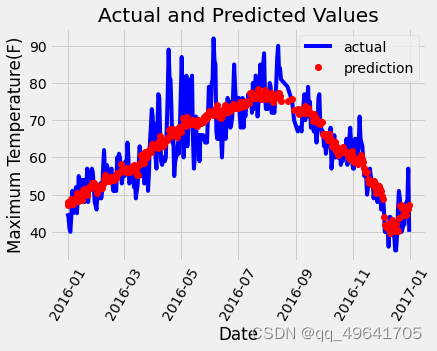
plt.plot(true_data['date'], true_data['actual'], 'b-', label = 'actual')#预测值
plt.plot(predictions_data['date'], predictions_data['prediction'], 'ro', label = 'prediction')
plt.xticks(rotation = '60')
plt.legend()
# 图名
plt.xlabel('Date');plt.ylabel('Maximum Temperature(F)');plt.title('Actual and Predicted Values');

结果如图所示，根据图示可以看出，预测结果基本符合变化趋势，而且也没有完全符合真实值，没有过拟合。