MSBD5003 Project1.0: Decision Tree Model

这次主要复现C4.5决策树算法，使用其预测酒店是否退订的问题。基于决策树，其核心思想是：根据信息增益选取每次的分支。相比id3，信息增益函数选取的更科学了。本文欲手把手从id3一点一点复现该决策树。附一些读取数据的代码（如果需要的话）

from pyspark.sql.functions import *
from pyspark.sql.types import *
from pyspark.sql import SparkSession
from math import logfilePath = './data/Hotel Reservations.csv/'
data = spark.read.csv(filePath, header=True, inferSchema=True)
data = data.select(data.columns[1:])	#id没有帮助
data.printSchema()
data.count()

root
|-- Booking_ID: string (nullable = true)
|-- no_of_adults: integer (nullable = true)
|-- no_of_children: integer (nullable = true)
|-- no_of_weekend_nights: integer (nullable = true)
|-- no_of_week_nights: integer (nullable = true)
|-- type_of_meal_plan: string (nullable = true)
|-- required_car_parking_space: integer (nullable = true)
|-- room_type_reserved: string (nullable = true)
|-- lead_time: integer (nullable = true)
|-- arrival_year: integer (nullable = true)
|-- arrival_month: integer (nullable = true)
|-- arrival_date: integer (nullable = true)
|-- market_segment_type: string (nullable = true)
|-- repeated_guest: integer (nullable = true)
|-- no_of_previous_cancellations: integer (nullable = true)
|-- no_of_previous_bookings_not_canceled: integer (nullable = true)
|-- avg_price_per_room: double (nullable = true)
|-- no_of_special_requests: integer (nullable = true)
|-- booking_status: string (nullable = true)

1. 前置工作：信息熵

1.1 信息熵的定义

把数据看做随机变量的话，信息熵是用来度量这个随机变量所包含的信息量或不确定性的指标。其计算公式为：
$$H=-\sum p(x_i)lo{g}_{2}p(x_i)$$
对于不确定性，我们自然是希望它越小越好。举个简单的例子，我们数据中booking status是我们最终要预测的指标，其按照canceled,not canceled可以分为两类即 X = { x 1 , x 2 } X=\{x_1,x_2\} X={x1​,x2​}一共有两种取值。我们想要计算信息熵显然就需要先统计两情况分别出现的次数，用频率去近似概率
$$频率（24390，11885）=》概率(0.6723,0.3277)$$
分别带入就以求得信息熵为:
$$H=-(0.6723\ast \log 0.6723+0.3277\ast \log 0.3277)=-0.9124$$
在pyspark中求解如下：

label_col='booking_status'
def entropy(data, label_col):n = data.count()label_freqs = data.groupBy(label_col).agg(count("*").alias("freq"))label_freqs = label_freqs.withColumn("prob", col("freq") / n)    print(label_freqs.collect())entropy = (label_freqs.selectExpr("prob * log2(prob) as product").selectExpr("-1 * sum(product) as entropy").first()["entropy"])print('Entropy in this class:',entropy)return entropy
a = entropy(data, label_col)
a

[Row(booking_status=‘Not_Canceled’, freq=24390, prob=0.6723638869745003), Row(booking_status=‘Canceled’, freq=11885, prob=0.32763611302549966)]
Entropy in this class: 0.9124929479549403

1.2 信息增益的定义

1.2.1 单个属性的信息增益

现在我们引入其他的变量信息，例如required_car_parking_space：0/1。相当于我们同时获得了这3w条信息的两条属性！那信息熵的计算发生了什么样的变化呢？

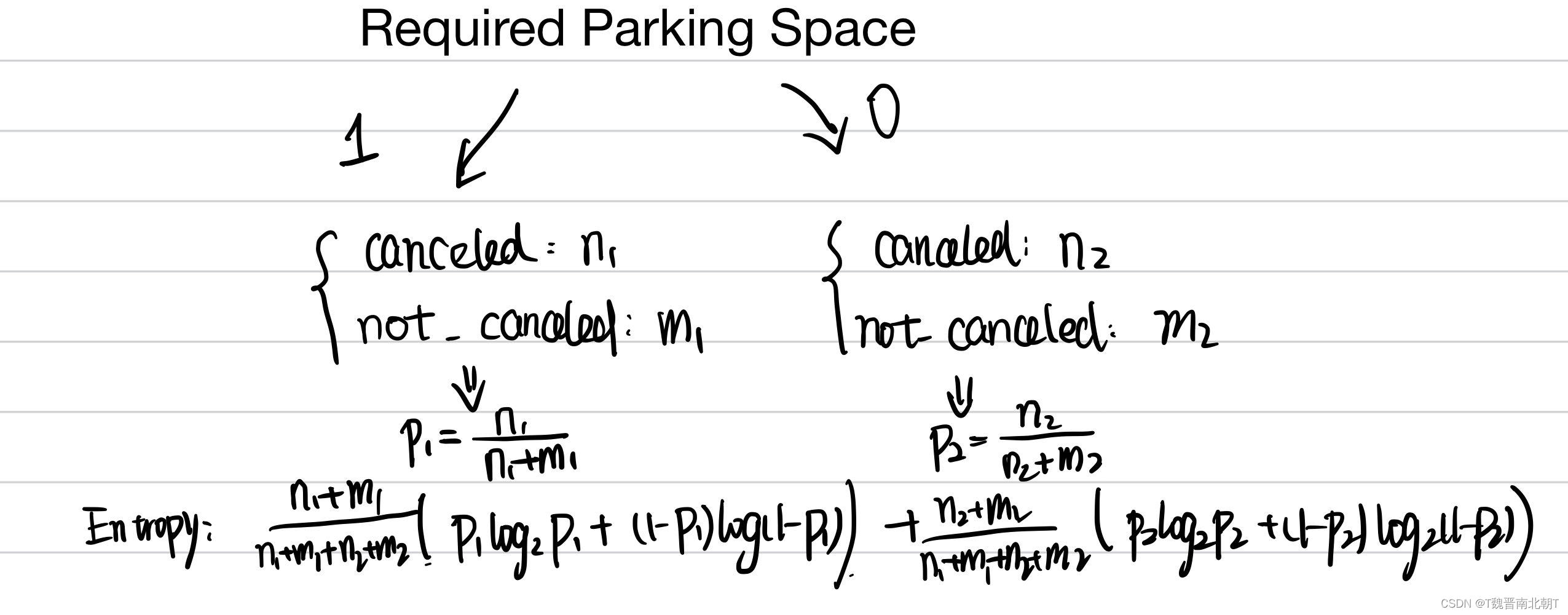
按照这条属性将信息分类后，不难发现我们可以继续在每类中按照我们的目标booking status继续计算信息熵，最后再把两类中各自的信息熵按照一定的权重合在一起就好。
这样分类后的信息熵和之前相比按道理来说应该是有区别的，在这里实现的代码和结果如下：

data1 = data.filter("required_car_parking_space='1'")
data0 = data.filter("required_car_parking_space='0'")
test_result0 = entropy(data0, label_col)
test_result1 = entropy(data1, label_col)
final_entropy = (data0.count()*test_result0+data1.count()*test_result1)/(data0.count()+data1.count())
final_entropy 

[Row(booking_status=‘Not_Canceled’, freq=23380, prob=0.6651304372564081), Row(booking_status=‘Canceled’, freq=11771, prob=0.3348695627435919)]
Entropy in this class: 0.9198244086154951
[Row(booking_status=‘Not_Canceled’, freq=1010, prob=0.8985765124555161), Row(booking_status=‘Canceled’, freq=114, prob=0.10142348754448399)]
Entropy in this class: 0.47349176948219907
0.905994556475293

不难发现，通过分组计算信息熵的方法得到的信息熵0.90确实比0.91降低了，那优化出来的0.1就是它的信息增益，说明用它来做根节点把数据集分开确实有效果。但是我们想要最好的哪一个，别的指标我们还没试过，怎么知道这个最好呢？本着兼听则明的心态，我们不如把所有的指标都比较一遍。所以上面的函数写的就太死了，需要能传入待split的指标。改进一下写法：

split_col = 'required_car_parking_space'
def information_gain(data, split_col, label_col):ex_entropy = entropy(data, label_col)groups = data.groupBy(split_col).agg(count("*").alias("count")).collect()n = data.count()gain = ex_entropyfor group in groups:print('*************entropy:',str(group[0]))a = data.filter(col(split_col) == str(group[0]))group_entropy = entropy(data.filter(col(split_col) == str(group[0])), label_col)group_weight = group[1] / ngain -= group_weight * group_entropyreturn gain
b = information_gain(data, split_col, label_col)
b

计算出来的信息增益为：

0.006498391479647148

1.2.2 多个信息增益的计算和比较

columns=data.columns[:-1]   #拿所有预测属性遍历一下
gains = [(col, information_gain(data, col, label_col)) for col in columns]

1.3 决策树的搭建

1.3.1 定义节点类

# 定义一个节点类，用来表示决策树的节点
class TreeNode(object):def __init__(self, feature=None, value=None, result=None):self.feature = feature   # 该节点的特征名称self.value = value       # 该节点的特征取值self.result = result     # 如果是叶子节点，表示预测结果self.children = []       # 该节点的子节点

1.3.2 判断结束的条件

显然，我们只想了第一步，在初始属性中找一个最好的作为根节点，例如我们根据某一属性，将数据分为了三组，然后呢？

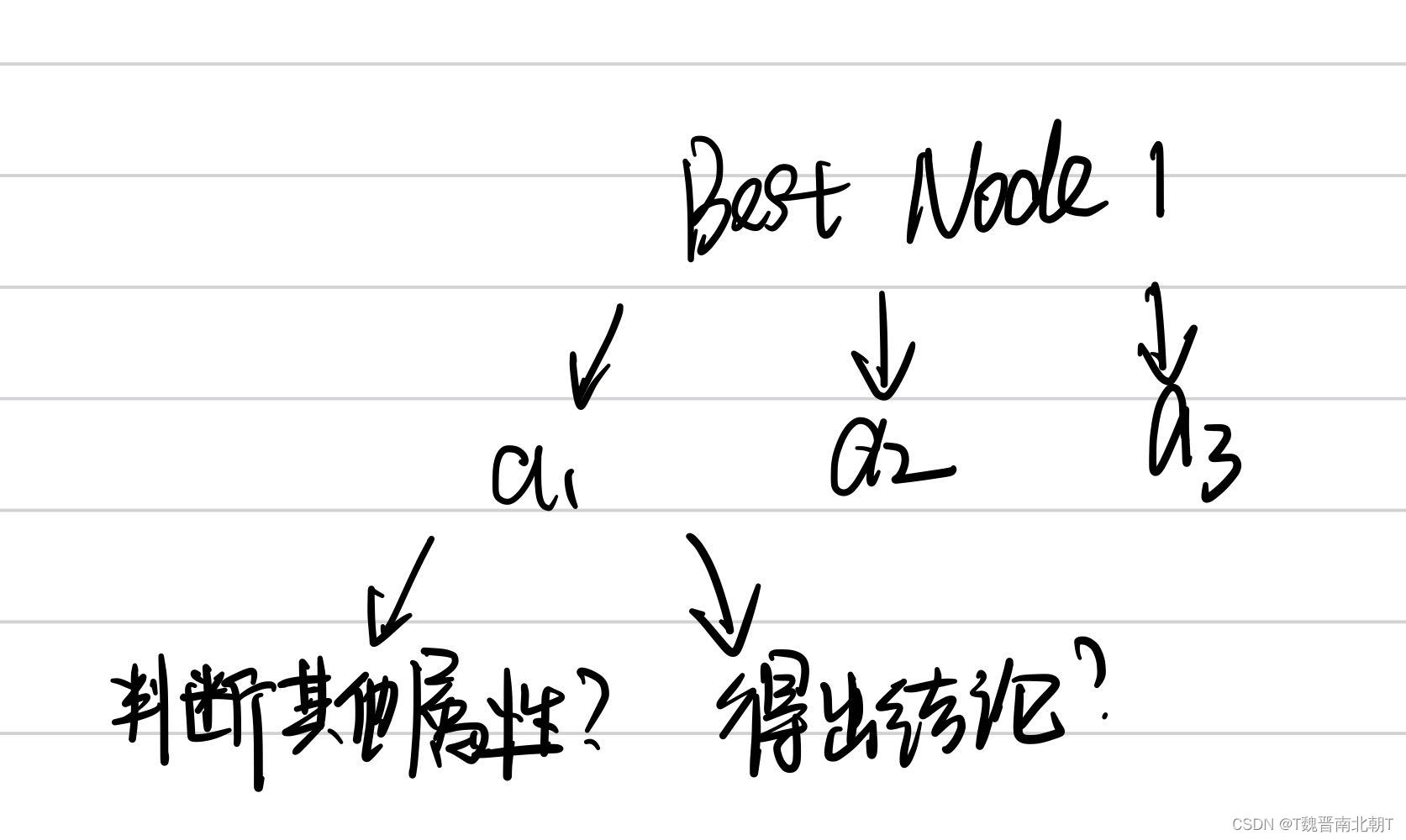
不难发现我们遇到了两个问题：

• 分组后我并没有直接因此得到想要预测的结果，我仍然还不知道对于每一组应该做出怎样的预测；
  Answer：这个显然可以想到，我使用组内样本出现最多的类别，少数服从多数。
• 对于已经得到的分组，我也不知道是需要进一步细分。
  Answer：这个问题就有些棘手，因为我们想让决策树分的足够细枝准确，又不想它给每种情况分一类引起过拟合，在不考虑进行剪枝的情况下我们可以从下面两个角度入手结束继续细分我们的组：

1. 如果当前的样本已经属于同一类别，无需继续分裂；
2. 信息增益是否足够高，如果小于设定阈值，就停止分裂。
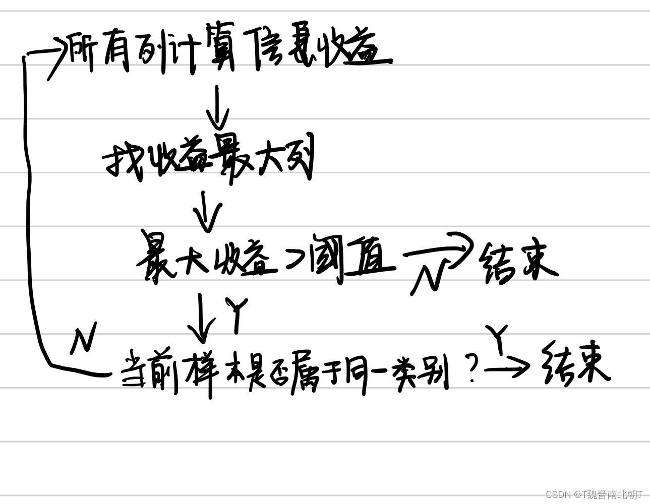
   把上面的思路落实一下就是下面的一段代码：

def build_tree(data, label_col, columns):# 初始化根节点n = data.count()label_freqs = data.groupBy(label_col).agg(count("*").alias("freq"))label_freqs = label_freqs.withColumn("freq_ratio", col("freq") / n)result = label_freqs.orderBy(desc("freq_ratio")).first()[label_col]if len(columns) == 0:return TreeNode(result=result)gains = [(col, information_gain(data, col, label_col)) for col in columns]best_col, best_gain = sorted(gains, key=lambda x: x[1], reverse=True)[0]if best_gain <= 0:        #这里设置阈值为0return TreeNode(result=result)new_columns = [col for col in columns if col != best_col]if len(new_columns) == 0:return TreeNode(result=result)print(new_columns)groups = data.groupBy(best_col).agg(count("*").alias("count"))node = TreeNode(feature=best_col)# 对子节点递归调用此生成算法for group in groups.collect():value = group[0]sub_data = data.filter(col(best_col) == value).drop(best_col)if sub_data.count() == 0:child = TreeNode(result=result)else:child = build_tree(sub_data, label_col, new_columns)child.value = valuenode.children.append(child)return node

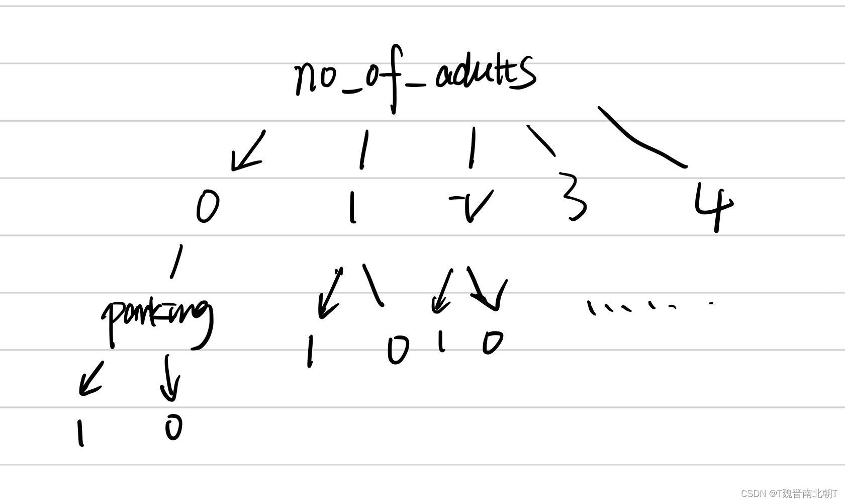
截止到目前我们终于学会1+1=2了，真不容易，赶紧选两个指标测试一下我们1+1=‘2’的实验效果，这次我们选取的指标为刚才讨论的parking和第一列adults：

columns=data.columns[:1]
columns.append('required_car_parking_space')
columns

[‘no_of_adults’, ‘required_car_parking_space’]

运行上面的代码就可以构造一颗决策树了，树最大的深度为2，构造出来的树长这个样子：

1.4 决策树的测试

试试我们这个小决策树能不能做出预测：

def predict(row, node):for child in node.children:if child.result is not None:return child.resultif row[child.feature] == child.value:return predict(row, child)
row = data.selectExpr("no_of_adults","required_car_parking_space").first()
a = predict(row, res)

‘Not_Canceled’

回去对着原表一看，蒙对了，还不错，这个ID3简易版就算是让我们搭好了，下面我们要做的东西：

• 使用C4.5，使用更好的信息增益的计算方法；
• 改进预测函数，能对多组输入一起进行预测；
• 将数据分为训练集和预测集，进行正式的训练；
• 考察数据的性质，进行适当清洗，以控制树的大小及提高树的准确率。