本文主要是介绍Autoleaders-数据分析pandas,希望对大家解决编程问题提供一定的参考价值,需要的开发者们随着小编来一起学习吧!
series
默认索引
import pandas as pd
import numpy as np
data = np.array(['a','b','c','d'])
s = pd.Series(data)
print (s)
0   a
1   b
2   c
3   d
dtype: object
指定索引
import pandas as pd
import numpy as np
data = np.array(['a','b','c','d'])
#自定义索引标签(即显示索引)
s = pd.Series(data,index=[100,101,102,103])
print(s)
100  a
101  b
102  c
103  d
dtype: object
字典创建
import pandas as pd
import numpy as np
data = {'a' : 0., 'b' : 1., 'c' : 2.}
s = pd.Series(data,index=['b','c','d','a'])
print(s)
b 1.0
c 2.0
d NaN
a 0.0
dtype: float64
切片
import pandas as pd
s = pd.Series([1,2,3,4,5],index = ['a','b','c','d','e'])
print(s[:3])
a  1
b  2
c  3
dtype: int64
import pandas as pd
s = pd.Series([6,7,8,9,10],index = ['a','b','c','d','e'])
print(s[['a','c','d']])
a 6
c 8
d 9
dtype: int64head,tail
import pandas as pd
import numpy as np
s = pd.Series(np.random.randn(5))
print ("The original series is:")
print (s)
#返回前三行数据
print (s.head(3))
原系列输出结果:
0    1.249679
1    0.636487
2   -0.987621
3    0.999613
4    1.607751
head(3)输出:
dtype: float64
0    1.249679
1    0.636487
2   -0.987621
dtype: float64
import pandas as pd
import numpy as np
s = pd.Series(np.random.randn(4))
#原series
print(s)
#输出后两行数据
print (s.tail(2))
原Series输出:
0 0.053340
1 2.165836
2 -0.719175
3 -0.035178
输出后两行数据:
dtype: float64
2 -0.719175
3 -0.035178
dtype: float64isnull,notnull
import pandas as pd
#None代表缺失数据
s=pd.Series([1,2,5,None])
print(pd.isnull(s))  #是空值返回True
print(pd.notnull(s)) #空值返回False
0    False
1    False
2    False
3     True
dtype: boolnotnull():
0     True
1     True
2     True
3    False
dtype: bool
DataFrame
创建
import pandas as pd
data = [['Alex',10],['Bob',12],['Clarke',13]]
df = pd.DataFrame(data,columns=['Name','Age'])
print(df)Name      Age
0     Alex      10
1     Bob       12
2     Clarke    13
import pandas as pd
data = [['Alex',10],['Bob',12],['Clarke',13]]
df = pd.DataFrame(data,columns=['Name','Age'],dtype=float)
print(df)Name Age
0 Alex 10.0
1 Bob 12.0
2 Clarke 13.0import pandas as pd
data = {'Name':['Tom', 'Jack', 'Steve', 'Ricky'],'Age':[28,34,29,42]}
df = pd.DataFrame(data, index=['rank1','rank2','rank3','rank4'])
print(df)Age Name
rank1 28 Tom
rank2 34 Jack
rank3 29 Steve
rank4 42 Rickyimport pandas as pd
data = [{'a': 1, 'b': 2},{'a': 5, 'b': 10, 'c': 20}]
df1 = pd.DataFrame(data, index=['first', 'second'], columns=['a', 'b'])
df2 = pd.DataFrame(data, index=['first', 'second'], columns=['a', 'b1'])
print(df1)
print(df2)
#df2输出a b
first 1 2
second 5 10#df1输出a b1
first 1 NaN
second 5 NaNimport pandas as pd
d = {'one' : pd.Series([1, 2, 3], index=['a', 'b', 'c']),'two' : pd.Series([1, 2, 3, 4], index=['a', 'b', 'c', 'd'])}
df = pd.DataFrame(d)
print(df)one two
a 1.0 1
b 2.0 2
c 3.0 3
d NaN 4读取
import pandas as pd
#需要注意文件的路径
df=pd.read_csv("C:/Users/Administrator/Desktop/person.csv",encoding="gbk")#读取的文件有中文时要加入最后这个
print (df)ID   Name  Age      City  Salary
0   1   Jack   28   Beijing   22000
1   2   Lida   32  Shanghai   19000
2   3   John   43  Shenzhen   12000
3   4  Helen   38  Hengshui    3500
import pandas as pd
#读取excel数据
df = pd.read_excel('website.xlsx',index_col='name',skiprows=[2])
#处理未命名列
df.columns = df.columns.str.replace('Unnamed.*', 'col_label')
print(df)col_label rank language agelimit
name
编程帮 0 1 PHP www.bianchneg.com
微学苑 2 3 PHP www.weixueyuan.com
92python 3 4 Python www.92python.com读取前三列
import pandas as pd
#读取excel数据
#index_col选择前两列作为索引列
#选择前三列数据,name列作为行索引
df = pd.read_excel('website.xlsx',index_col='name',index_col=[0,1],usecols=[1,2,3])
#处理未命名列,固定用法
df.columns = df.columns.str.replace('Unnamed.*', 'col_label')
print(df)language
name      rank
编程帮       1          PHP
c语言中文网   2           C
微学苑       3          PHP
92python    4         Python
索引
import pandas as pd
d = {'one' : pd.Series([1, 2, 3], index=['a', 'b', 'c']),'two' : pd.Series([1, 2, 3, 4], index=['a', 'b', 'c', 'd'])}
df = pd.DataFrame(d)
print(df ['one'])
a     1.0
b     2.0
c     3.0
d     NaN
Name: one, dtype: float64
import pandas as pd
d = {'one' : pd.Series([1, 2, 3], index=['a', 'b', 'c']),'two' : pd.Series([1, 2, 3, 4], index=['a', 'b', 'c', 'd'])}
df = pd.DataFrame(d)
print(df.loc['b'])
one 2.0two 2.0Name: b, dtype: float64添加,删除
import pandas as pd
d = {'one' : pd.Series([1, 2, 3], index=['a', 'b', 'c']),'two' : pd.Series([1, 2, 3, 4], index=['a', 'b', 'c', 'd'])}
df = pd.DataFrame(d)
#使用df['列']=值,插入新的数据列
df['three']=pd.Series([10,20,30],index=['a','b','c'])
print(df)
#将已经存在的数据列做相加运算
df['four']=df['one']+df['three']
print(df)
使用列索引创建新数据列:one   two   three
a    1.0    1    10.0
b    2.0    2    20.0
c    3.0    3    30.0
d    NaN    4    NaN已存在的数据列做算术运算:one   two   three    four
a     1.0    1    10.0     11.0
b     2.0    2    20.0     22.0
c     3.0    3    30.0     33.0
d     NaN    4     NaN     NaN
import pandas as pd
d = {'one' : pd.Series([1, 2, 3], index=['a', 'b', 'c']),'two' : pd.Series([1, 2, 3, 4], index=['a', 'b', 'c', 'd'])}
df = pd.DataFrame(d)
print (df.iloc[2])
one 3.0
two 3.0
Name: c, dtype: float64import pandas as pd
d = {'one' : pd.Series([1, 2, 3], index=['a', 'b', 'c']),'two' : pd.Series([1, 2, 3, 4], index=['a', 'b', 'c', 'd'])}
df = pd.DataFrame(d)
#左闭右开
print(df[2:4])one two
c 3.0 3
d NaN 4import pandas as pd
info=[['Jack',18],['Helen',19],['John',17]]
df=pd.DataFrame(info,columns=['name','age'])
print(df)
#注意是column参数
#数值1代表插入到columns列表的索引位置
df.insert(1,column='score',value=[91,90,75])
print(df)
添加前:name age
0 Jack 18
1 Helen 19
2 John 17添加后:name score age
0 Jack 91 18
1 Helen 90 19
2 John 75 17import pandas as pd
d = {'one' : pd.Series([1, 2, 3], index=['a', 'b', 'c']),'two' : pd.Series([1, 2, 3, 4], index=['a', 'b', 'c', 'd']),'three' : pd.Series([10,20,30], index=['a','b','c'])}
df = pd.DataFrame(d)
print ("Our dataframe is:")
print(df)
#使用del删除
del df['one']
print(df)
#使用pop方法删除
df.pop('two')
print (df)
原DataFrame:one three two
a 1.0 10.0 1
b 2.0 20.0 2
c 3.0 30.0 3
d NaN NaN 4使用del删除 first:three two
a 10.0 1
b 20.0 2
c 30.0 3
d NaN 4使用 pop()删除:three
a 10.0
b 20.0
c 30.0
d NaNimport pandas as pd
df = pd.DataFrame([[1, 2], [3, 4]], columns = ['a','b'])
df2 = pd.DataFrame([[5, 6], [7, 8]], columns = ['a','b'])
#在行末追加新数据行
df = df.append(df2)
print(df)a b
0 1 2
1 3 4
0 5 6
1 7 8import pandas as pd
df = pd.DataFrame([[1, 2], [3, 4]], columns = ['a','b'])
df2 = pd.DataFrame([[5, 6], [7, 8]], columns = ['a','b'])
df = df.append(df2)
print(df)
#注意此处调用了drop()方法
df = df.drop(0)
print (df)
执行drop(0)前:a b
0 1 2
1 3 4
0 5 6
1 7 8执行drop(0)后:a b
1 3 4
1 7 8求值
sum()和
import pandas as pd
import numpy as np
#创建字典型series结构
d = {'Name':pd.Series(['小明','小亮','小红','小华','老赵','小曹','小陈','老李','老王','小冯','小何','老张']),'Age':pd.Series([25,26,25,23,30,29,23,34,40,30,51,46]),'Rating':pd.Series([4.23,3.24,3.98,2.56,3.20,4.6,3.8,3.78,2.98,4.80,4.10,3.65])
}
df = pd.DataFrame(d)
#默认axis=0或者使用sum("index")
print(df.sum())
Name      小明小亮小红小华老赵小曹小陈老李老王小冯小何老张
Age                            382
Rating                       44.92
dtype: object
import pandas as pd
import numpy as np
d = {'Name':pd.Series(['小明','小亮','小红','小华','老赵','小曹','小陈','老李','老王','小冯','小何','老张']),'Age':pd.Series([25,26,25,23,30,29,23,34,40,30,51,46]),'Rating':pd.Series([4.23,3.24,3.98,2.56,3.20,4.6,3.8,3.78,2.98,4.80,4.10,3.65])
}
df = pd.DataFrame(d)
#也可使用sum("columns")或sum(1)
print(df.sum(axis=1))
0 29.23
1 29.24
2 28.98
3 25.56
4 33.20
5 33.60
6 26.80
7 37.78
8 42.98
9 34.80
10 55.10
11 49.65
dtype: float64mean()平均值
import pandas as pd
import numpy as np
d = {'Name':pd.Series(['小明','小亮','小红','小华','老赵','小曹','小陈','老李','老王','小冯','小何','老张']),'Age':pd.Series([25,26,25,23,30,29,23,34,40,30,51,46]),'Rating':pd.Series([4.23,3.24,3.98,2.56,3.20,4.6,3.8,3.78,2.98,4.80,4.10,3.65])
}
df = pd.DataFrame(d)
print(df.mean())
Age       31.833333
Rating     3.743333
dtype: float64
std()标准差
import pandas as pd
import numpy as np
d = {'Name':pd.Series(['小明','小亮','小红','小华','老赵','小曹','小陈','老李','老王','小冯','小何','老张']),'Age':pd.Series([25,26,25,23,59,19,23,44,40,30,51,54]),'Rating':pd.Series([4.23,3.24,3.98,2.56,3.20,4.6,3.8,3.78,2.98,4.80,4.10,3.65])
}
df = pd.DataFrame(d)
print(df.std())
Age       13.976983
Rating     0.661628
dtype: float64
describe()数据汇总
import pandas as pd
import numpy as np
d = {'Name':pd.Series(['小明','小亮','小红','小华','老赵','小曹','小陈','老李','老王','小冯','小何','老张']),'Age':pd.Series([25,26,25,23,30,29,23,34,40,30,51,46]),'Rating':pd.Series([4.23,3.24,3.98,2.56,3.20,4.6,3.8,3.78,2.98,4.80,4.10,3.65])
}
#创建DataFrame对象
df = pd.DataFrame(d)
#求出数据的所有描述信息
print(df.describe())Age     Rating
count  12.000000  12.000000
mean   34.916667   3.743333
std    13.976983   0.661628
min    19.000000   2.560000
25%    24.500000   3.230000
50%    28.000000   3.790000
75%    45.750000   4.132500
max    59.000000   4.800000
import pandas as pd
import numpy as np
d = {'Name':pd.Series(['小明','小亮','小红','小华','老赵','小曹','小陈','老李','老王','小冯','小何','老张']),'Age':pd.Series([25,26,25,23,59,19,23,44,40,30,51,54]),'Rating':pd.Series([4.23,3.24,3.98,2.56,3.20,4.6,3.8,3.78,2.98,4.80,4.10,3.65])
}
df = pd.DataFrame(d)
print(df.describe(include=["object"]))Name
count 12
unique 12
top 小红
freq 1import pandas as pd
import numpy as np
d = {'Name':pd.Series(['小明','小亮','小红','小华','老赵','小曹','小陈','老李','老王','小冯','小何','老张']),'Age':pd.Series([25,26,25,23,59,19,23,44,40,30,51,54]),'Rating':pd.Series([4.23,3.24,3.98,2.56,3.20,4.6,3.8,3.78,2.98,4.80,4.10,3.65])
}
df = pd.DataFrame(d)
print(df.describe(include="all"))Name Age Rating
count 12 12.000000 12.000000
unique 12 NaN NaN
top 小红 NaN NaN
freq 1 NaN NaN
mean NaN 34.916667 3.743333
std NaN 13.976983 0.661628
min NaN 19.000000 2.560000
25% NaN 24.500000 3.230000
50% NaN 28.000000 3.790000
75% NaN 45.750000 4.132500
max NaN 59.000000 4.800000转化
import pandas as pd
data = {'Name': ['Smith', 'Parker'], 'ID': [101, 102], 'Language': ['Python', 'JavaScript']}
info = pd.DataFrame(data)
print('DataFrame Values:\n', info)
#转换为csv数据
csv_data = info.to_csv()
print('\nCSV String Values:\n', csv_data)
DataFrame:Name   ID    Language
0   Smith  101      Python
1  Parker  102  JavaScriptcsv数据:
,Name,ID,Language
0,Smith,101,Python
1,Parker,102,JavaScript
import pandas as pd
#注意:pd.NaT表示null缺失数据
data = {'Name': ['Smith', 'Parker'], 'ID': [101, pd.NaT], 'Language': ['Python', 'JavaScript']}
info = pd.DataFrame(data)
csv_data = info.to_csv("C:/Users/Administrator/Desktop/pandas.csv",sep='|')import pandas as pd
#创建DataFrame数据
info_website = pd.DataFrame({'name': ['编程帮', 'c语言中文网', '微学苑', '92python'],'rank': [1, 2, 3, 4],'language': ['PHP', 'C', 'PHP','Python' ],'url': ['www.bianchneg.com', 'c.bianchneg.net', 'www.weixueyuan.com','www.92python.com' ]})
#创建ExcelWrite对象
writer = pd.ExcelWriter('website.xlsx')
info_website.to_excel(writer)
writer.save()
print('输出成功')growby分组
import pandas as pdsales = pd.read_csv("sales_data.csv")sales.head()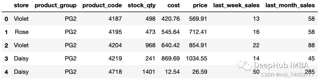
单列聚合
sales.groupby("store")["stock_qty"].mean()#输出storeDaisy 1811.861702Rose 1677.680000Violet 14622.406061Name: stock_qty, dtype: float64
多列聚合
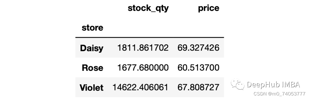
sales.groupby("store")[["stock_qty","price"]].mean()
多列多个聚合
sales.groupby("store")["stock_qty"].agg(["mean", "max"])

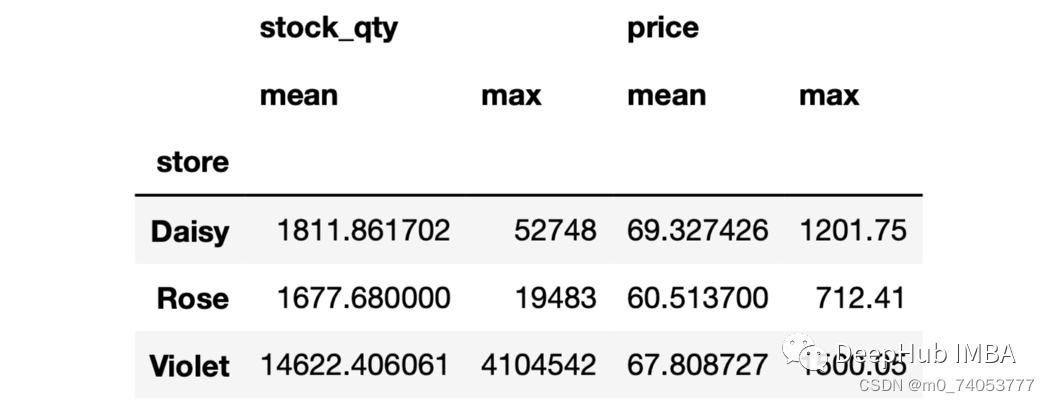
sales.groupby("store")[["stock_qty","price"]].agg(["mean", "max"])
命名
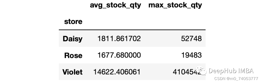
sales.groupby("store").agg( avg_stock_qty = ("stock_qty", "mean"),max_stock_qty = ("stock_qty", "max"))
sales.groupby("store").agg(avg_stock_qty = ("stock_qty", "mean"),avg_price = ("price", "mean"))

as_index
sales.groupby("store", as_index=False).agg(avg_stock_qty = ("stock_qty", "mean"),avg_price = ("price", "mean"))

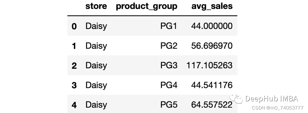
sales.groupby(["store","product_group"], as_index=False).agg(avg_sales = ("last_week_sales", "mean")).head()
sort_values
sales.groupby(["store","product_group"], as_index=False).agg( avg_sales = ("last_week_sales", "mean")).sort_values(by="avg_sales", ascending=False).head()
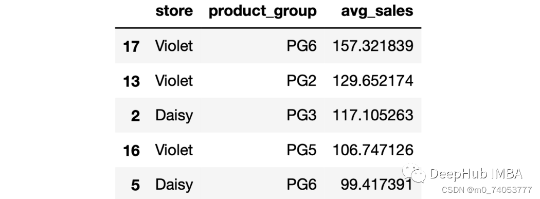
sales.groupby(["store","product_group"], as_index=False).agg( avg_sales = ("last_week_sales", "mean")).sort_values(by="avg_sales", ascending=False).head()

nlargest
sales.groupby("store")["last_week_sales"].nlargest(2)store Daisy 413 1883231 947Rose 948 883263 623Violet 991 3222339 2690Name: last_week_sales, dtype: int64
nsmallest
sales.groupby("store")["last_week_sales"].nsmallest(2)
nth
sales_sorted = sales.sort_values(by=["store","last_month_sales"], ascending=False, ignore_index=True)
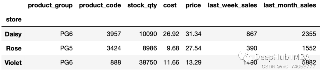
sales_sorted.groupby("store").nth(4)
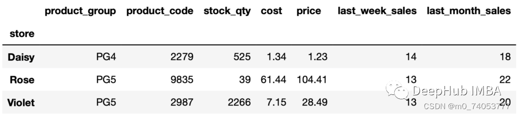
sales_sorted.groupby("store").nth(-2)
unique
sales.groupby("store", as_index=False).agg(unique_values = ("product_code","unique"))

sales.groupby("store", as_index=False).agg(number_of_unique_values = ("product_code","nunique"))

lambda
sales.groupby("store").agg(total_sales_in_thousands = ("last_month_sales",lambda x: round(x.sum() / 1000, 1)))

apply
sales.groupby("store").apply(lambda x: (x.last_week_sales - x.last_month_sales / 4).mean())storeDaisy 5.094149Rose 5.326250Violet 8.965152dtype: float64
dropna
无dropna
sales.loc[1000] = [None, "PG2", 10000, 120, 64, 96, 15, 53]
sales.groupby("store")["price"].mean()storeDaisy     69.327426Rose     60.513700Violet   67.808727Name: price, dtype: float64
有dropna
sales.groupby("store", dropna=False)["price"].mean()storeDaisy 69.327426Rose 60.513700Violet 67.808727NaN 96.000000Name: price, dtype: float64
ngroups
sales.groupby(["store", "product_group"]).ngroups18
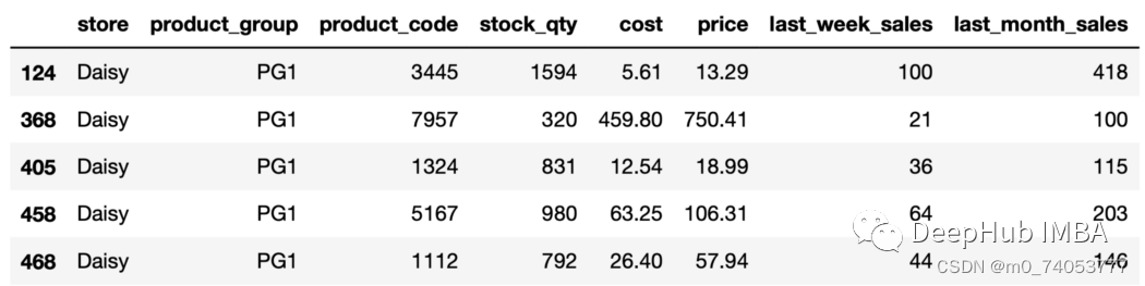
get_group
aisy_pg1 = sales.groupby(["store", "product_group"]).get_group(("Daisy","PG1"))daisy_pg1.head()
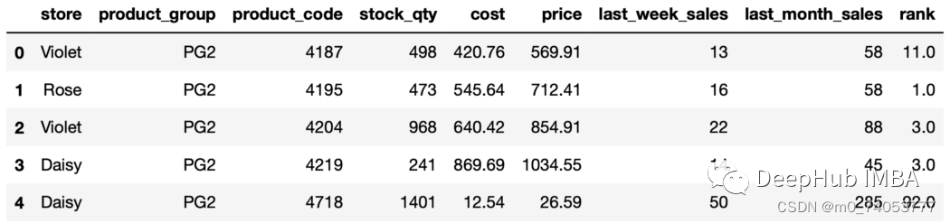
rank
sales["rank"] = sales.groupby("store"["price"].rank(ascending=False, method="dense")sales.head()
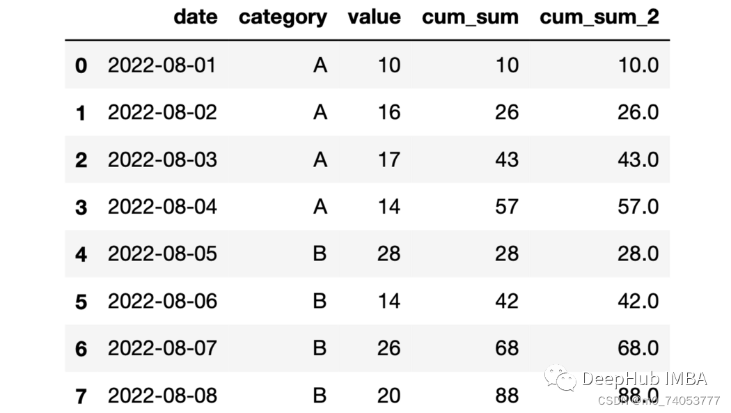
cumsum
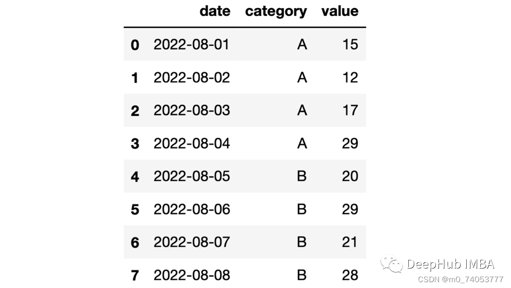
import numpy as npdf = pd.DataFrame({"date": pd.date_range(start="2022-08-01", periods=8, freq="D"),"category": list("AAAABBBB"),"value": np.random.randint(10, 30, size=8)})
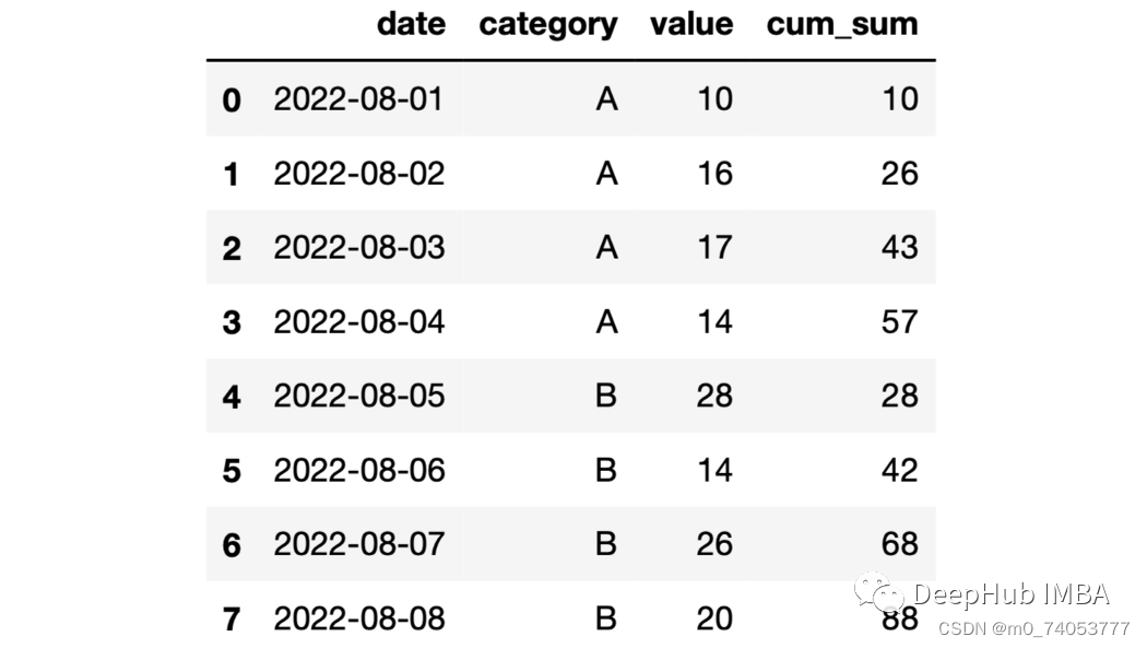
df["cum_sum"] = df.groupby("category")["value"].cumsum()
expanding
df["cum_sum_2"] = df.groupby("category")["value"].expanding().sum().values
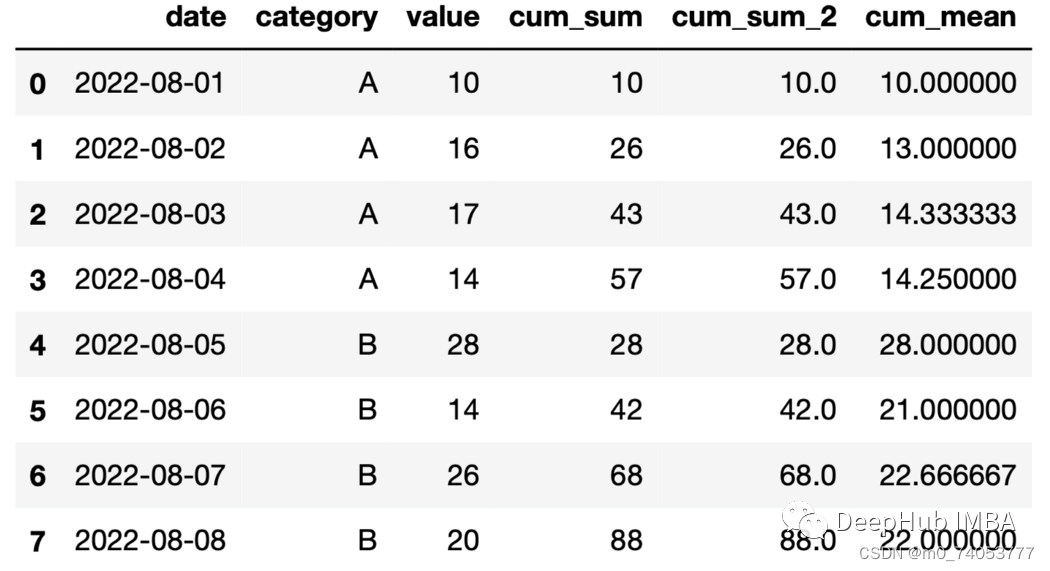
expanding+mean累计平均
df["cum_mean"] = df.groupby("category")["value"].expanding().mean().values
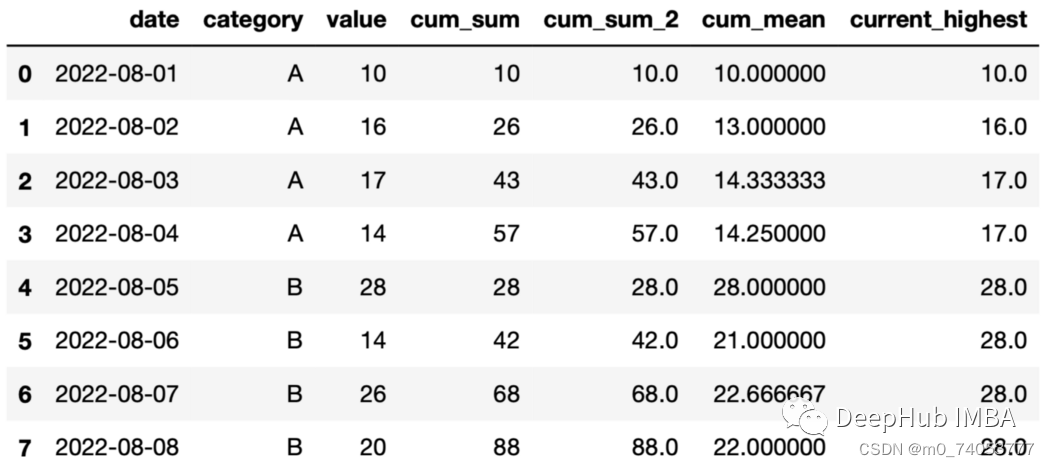
expand+max
df["current_highest"] = df.groupby("category")["value"].expanding().max().values
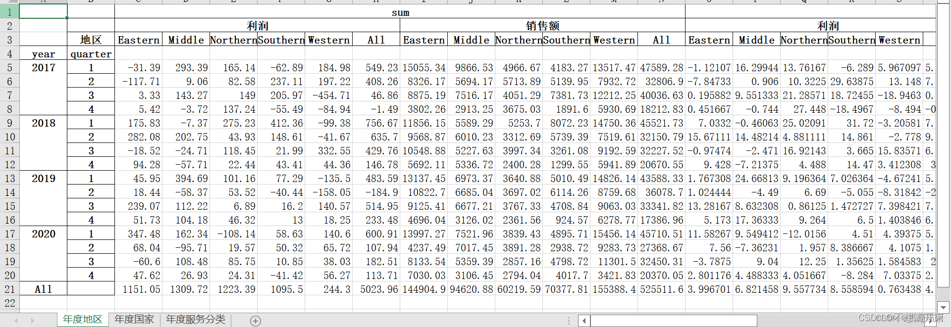
pivot_table()
ind=pd.DatetimeIndex(data01['日期'])
data01=data01.set_index(ind)
#分组
data01['year']=data01['日期'].dt.year
data01['quarter']=data01['日期'].dt.quarter
#统计各个年度/季度中,地区、国家、服务分类的销售额和利润数据writer = pd.ExcelWriter('result1.1.xlsx')
diqu=data01.pivot_table(['利润','销售额'],index=['year','quarter'],columns='地区',aggfunc=['sum','mean','median'],margins=True)
diqu.to_excel(writer,index=True,sheet_name='年度地区')
gj=data01.pivot_table(['利润','销售额'],index=['year','quarter'],columns='国家',aggfunc=['sum','mean','median'],margins=True)
gj.to_excel(writer,index=True,sheet_name='年度国家')
fw=data01.pivot_table(['利润','销售额'],index=['year','quarter'],columns='服务分类',aggfunc=['sum','mean','median'],margins=True)
fw.to_excel(writer,index=True,sheet_name='年度服务分类')writer.save()
writer.close()
shift
数据移动
>>> df = pd.DataFrame({"Col1": [10, 20, 15, 30, 45],"Col2": [13, 23, 18, 33, 48],"Col3": [17, 27, 22, 37, 52]},index=pd.date_range("2020-01-01", "2020-01-05"))
>>> dfCol1  Col2  Col3
2020-01-01    10    13    17
2020-01-02    20    23    27
2020-01-03    15    18    22
2020-01-04    30    33    37
2020-01-05    45    48    52
>>> df.shift(periods=3)  # 或df.shift(3)Col1  Col2  Col3
2020-01-01   NaN   NaN   NaN
2020-01-02   NaN   NaN   NaN
2020-01-03   NaN   NaN   NaN
2020-01-04  10.0  13.0  17.0
2020-01-05  20.0  23.0  27.0>>> df.shift(0)Col1  Col2  Col3
2020-01-01    10    13    17
2020-01-02    20    23    27
2020-01-03    15    18    22
2020-01-04    30    33    37
2020-01-05    45    48    52>>> df.shift(1) # 或df.shift()Col1  Col2  Col3
2020-01-01   NaN   NaN   NaN
2020-01-02  10.0  13.0  17.0
2020-01-03  20.0  23.0  27.0
2020-01-04  15.0  18.0  22.0
2020-01-05  30.0  33.0  37.0# 当前行 减 上一行
>>> df.shift(0) - df.shift(1)Col1  Col2  Col3
2020-01-01   NaN   NaN   NaN
2020-01-02  10.0  10.0  10.0
2020-01-03  -5.0  -5.0  -5.0
2020-01-04  15.0  15.0  15.0
2020-01-05  15.0  15.0  15.0
>>> df.shift(periods=1, axis="columns")Col1  Col2  Col3
2020-01-01   NaN    10    13
2020-01-02   NaN    20    23
2020-01-03   NaN    15    18
2020-01-04   NaN    30    33
2020-01-05   NaN    45    48
>>> df.shift(periods=3, fill_value=0)Col1  Col2  Col3
2020-01-01     0     0     0
2020-01-02     0     0     0
2020-01-03     0     0     0
2020-01-04    10    13    17
2020-01-05    20    23    27
排序
#按照多列排序
print(df.sort_values(by=['最高温度','最低温度'],ascending= True).head(10))
'''
打印:日期  最高温度  最低温度     天气   风向  风级 空气质量
363  2019/12/30    -5   -12      晴  西北风  4级    优
364  2019/12/31    -3   -10      晴  西北风  1级    优
42    2019/2/12    -3    -8  小雪~多云  东北风  2级    优
44    2019/2/14    -3    -6  小雪~多云  东南风  2级    良
14    2019/1/15    -2   -10      晴  西北风  3级    良
37     2019/2/7    -2    -7     多云  东北风  3级    优
38     2019/2/8    -1    -7     多云  西南风  2级    优
4      2019/1/5     0    -8     多云  东北风  2级    优
39     2019/2/9     0    -8     多云  东北风  2级    优
40    2019/2/10     0    -8     多云  东南风  1级    优
print(df.sort_values(by=['最高温度','最低温度'],ascending= False).head(10))
'''
打印:日期  最高温度  最低温度      天气   风向  风级  空气质量
184   2019/7/4    38    25    晴~多云  西南风  2级     良
206  2019/7/26    37    27       晴  西南风  2级     良
142  2019/5/23    37    21       晴  东南风  2级     良
201  2019/7/21    36    27    晴~多云  西南风  2级  轻度污染
204  2019/7/24    36    27  多云~雷阵雨  西南风  2级     良
207  2019/7/27    36    27      多云  东南风  2级  轻度污染
174  2019/6/24    36    24      多云  东南风  2级     良
175  2019/6/25    36    24      多云  东南风  2级     良
183   2019/7/3    36    24       晴  东南风  1级     良
170  2019/6/20    36    23    多云~晴  东南风  2级  轻度污染
print(df.sort_values(by=['最高温度','最低温度'],ascending= [True,False]).head(10))
'''
打印:日期  最高温度  最低温度     天气   风向  风级 空气质量
363  2019/12/30    -5   -12      晴  西北风  4级    优
44    2019/2/14    -3    -6  小雪~多云  东南风  2级    良
42    2019/2/12    -3    -8  小雪~多云  东北风  2级    优
364  2019/12/31    -3   -10      晴  西北风  1级    优
37     2019/2/7    -2    -7     多云  东北风  3级    优
14    2019/1/15    -2   -10      晴  西北风  3级    良
38     2019/2/8    -1    -7     多云  西南风  2级    优
4      2019/1/5     0    -8     多云  东北风  2级    优
39     2019/2/9     0    -8     多云  东北风  2级    优
40    2019/2/10     0    -8     多云  东南风  1级    优
这篇关于Autoleaders-数据分析pandas的文章就介绍到这儿,希望我们推荐的文章对编程师们有所帮助!


