chapter 1 formation of crystal, basic concepts

chapter 1 晶体的形成

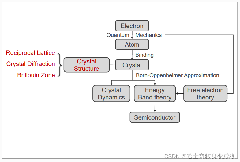
1.1 Quantum Mechanics and atomic structure

1.1.1 Old Quantum Theory

problems of planetary model:

• atom would be unstable
• radiate EM wave of continuous frequency

to solve the prablom of planetary model:

• Bohr: Quantum atomic structure
• Planck: Quantum

Old Quantum Theory: Planck, Einstein, Bohr, de Broglie

1. Planck’s theory: Each atomic oscillator can have only discrete values of energy. $E=nh\nu ,n=0,1,2,\dots$
2. Einstein: photon, $E=h\nu =\hslash \omega$, $p=\frac{E}{c}n=\frac{h\nu }{c}n=\frac{h}{\lambda }n=\hslash k$
3. Bohr: H atom model
4. de Broglie: Matter wave, $E=h\nu =\hslash \omega$,$E_k=\frac{1}{2}m{\nu }^2=\frac{p^2}{2m}=\frac{(\hslash k{)}^2}{2m}$

from de Broglie’s Hypothesis, the motion of a particle is governed by the wave propagation properties of matter wave, which means wave function.

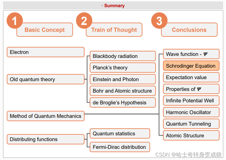
1.1.2 Method of Quantum Mechanics

In method of Quantum Mechanics, we should get the Schrodinger Equation and solve it, then find the wave function $\psi$.

Schrodinger Equation (very important):
$$i\hslash \frac{\partial \Psi }{\partial t}=-\frac{{\hslash }^2}{2m}{\nabla }^2\Psi +U\Psi$$

a. Schrodinger Equation of free particle

KaTeX parse error: Undefined control sequence: \pPsi at position 24: …\frac{\partial \̲p̲P̲s̲i̲}{\partial t}= …

wave function of free particle: $\psi (\vec{r},t)=A{e}^{-\frac{i}{\hslash }(Et-p\cdot r)}$

$$E⟶i\hslash \frac{\partial }{\partial t}$$

$$\mathbf{p}⟶-i\hslash \nabla$$

b. Schrodinger Equation of particle in a force field

$$i\hslash \frac{\partial \Psi }{\partial t}=-\frac{{\hslash }^2}{2m}{\nabla }^2\Psi +U\Psi$$

We consider time-independent Schrodinger Equation:

$$U(\mathbf{r},t)⟶U(\mathbf{r})$$

then separation of variables: KaTeX parse error: Undefined control sequence: \math at position 28: …f{r} ,t)= \psi(\̲m̲a̲t̲h̲{r})f(t)

Halmiton operator: $$\hat{H}=-\frac{{\hslash }^2}{2m}{\nabla }^2+U$$

so the Schrodinger Equ becomes a new style:

$$\hat{H}\psi =E\psi$$

$$\hat{H}\Psi =i\hslash \frac{\partial }{\partial t}\Psi$$

c. Infinite Potential Well

$$-(\frac{{\hslash }^2}{2m}\frac{d^2}{d{x}^2}+U(x))\psi (x)=E\psi (x)$$

$$\psi (x)=\sqrt{\frac{2}{a}}sin\frac{n\pi }{a}x$$

$$E=E_n=\frac{{\pi }^2{\hslash }^2}{2m{a}^2}{n}^2,n=1,2,3,\dots$$

d. Harmonic Oscillator 1D

$$-(\frac{{\hslash }^2}{2m}\frac{d^2}{d{x}^2}+\frac{1}{2}m{\omega }^2{x}^2)\psi (x)=E\psi (x)$$

$$E_n=(n+\frac{1}{2})\hslash \omega =(n+\frac{1}{2})h\nu ,n=0,1,2,3,\dots$$

• $E_{min}=\frac{1}{2}h\nu (\ne 0)$, which is different from Planck’s blackbody theory ($E=nh\nu ,E_{min}=0$)
• In classical mechanics, the particle can bot exceed x(max), but in quantum mechanics, the particle may exceed x(max) (qith low probabilities)

e. Finite Potential Well

$$(-\frac{{\hslash }^2}{2m}\frac{d^2}{d{x}^2}+U(x))\psi (x)=E\psi (x)$$

Quantum Tunneling

f. Atomic Structure, Schrodinger Equ. for H Atom

$$(-\frac{{\hslash }^2}{2m}{\nabla }^2+U)\psi =E\psi ,{\nabla }^2=\frac{{\partial }^2}{\partial x^2}+\frac{{\partial }^2}{\partial y^2}+\frac{{\partial }^2}{\partial z^2}$$

Schrodinger equ. becomes:

$$\frac{1}{r^2}\frac{\partial }{\partial r}(r^2\frac{\partial \psi }{\partial r})+\frac{1}{r^2\sin \theta }\frac{\partial }{\partial \theta }(\sin \theta \frac{\partial \psi }{\partial \theta })+\frac{1}{r^2{\sin }^2\theta }\frac{{\partial }^2\theta }{\partial {\varphi }^2}+\frac{2m}{\hslash }(E-U)\psi =0$$

use seperation of variables: $$\psi (r,\theta ,\varphi )=R(r)\Theta (\theta )\Phi (\varphi )$$

Schrodinger equ. becomes:

$$\frac{-{\sin }^2\theta }{R}\frac{d}{dr}(r^2\frac{dR}{dr})-\frac{2m}{{\hslash }^2}{r}^2{\sin }^2\theta (E-U)-\frac{\sin \theta }{\Theta }=0$$

Both Equal to a constant

$$\{\begin{array}{l}\frac{1}{\Phi }\frac{d^2\Phi }{d{\varphi }^2}=-m_l^2\\ \frac{m_l^2}{{\sin }^2\theta }-\frac{1}{\Theta }\frac{1}{\sin \theta }\frac{d}{d\theta }(\sin \theta \frac{d\Theta }{dtheta})=l(l+1)\\ \frac{1}{R}\frac{d}{dr}(r^2\frac{dR}{dr})+\frac{2m}{{\hslash }^2}{r}^2(E-U)=l(l+1)\end{array}$$

(1) $\varphi$ must be single-valued: $$m_l=0,\pm 1,\pm 2,\dots$$

(2) $\Theta$ must be finite: $$l=0,1,2,\dots andl\ge |m_l|$$

(3) R must be finite: $$E=E_n=-\frac{Z^2{e}^{4}m}{8{ϵ}_0^2{h}^2}\frac{1}{n^2},n=1,2,3,\dots andl<n$$

$$\{\begin{array}{l}主量子数n:principlequantumnumber⟶decide{E}_n\\ 角量子数l:orbitalquantumnumber⟶0,1,2,\dots ,n-1\\ 磁量子数m_l:magneticquantumnumber⟶0,\pm 1,\pm 2,\pm 3,\dots ,\pm l\end{array}$$

不考虑自旋，量子数=波函数个数=量子态数=轨道数

Pauli’s Exclusion Principle: not 2 electrons in a system ( an atom or a solid ) can be in the same quantum state ( have the same n, l, $m_l$, $m_s$)

1.1.3 Distributing functions of micro-particles

A system with N identical micro-particles, without either generation of new particles or vanishing of existed particles, without energy exchange—an isolated system

energy level: $$E_1,E_2,E_3,\dots ,E_l,\dots$$

degeneracy:$${\omega }_1,{\omega }_2,{\omega }_3,\dots .{\omega }_l,\dots$$

particle number: $$a_1,a_2,a_3,\dots ,a_l,\dots$$

全同性原理给量子统计和经典统计带来重要差别；
泡利不相容原理又给费米子和玻色子的统计带来重要差别。

自旋为$\pm \frac{1}{2}$的粒子服从泡利不相容原理。

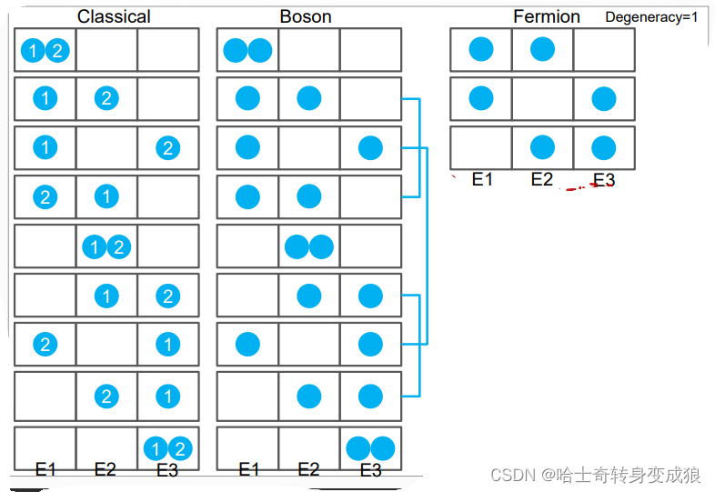
a. Boltzmann system

Every particle is identified, the number of particles in an quantum state is unlimited.

标号可分辨，能级上粒子数无限制

$$a_l=\frac{{\omega }_l}{e^{\alpha +\beta E_l}}$$

Boltzmann statistics: $$f_l=\frac{a_l}{{\omega }_l}=\frac{1}{e^{\alpha +\beta E_l}}=\frac{1}{e^{\frac{E_l-\mu }{k_{B}T}}}$$

b. Bose system

Every particle is unidentified, the number of particles in an quantum state is unlimited.

(photon,phonon…) - Boson

玻色子：声子、光子

不可分辨，能级上粒子无限

$$a_l=\frac{{\omega }_l}{e^{\alpha +\beta E_l}-1}$$

Bose-Einstein statistics: $$f_l=\frac{a_l}{{\omega }_l}=\frac{1}{e^{\alpha +\beta E_l}-1}=\frac{1}{e^{\frac{E_l-\mu }{k_{B}T}}-1}$$

c.Femi system

Every particle is unidentified, the number of particles in an quantum state is limited by Pauli repulsive principle.

(electron, proton…) - Fermion

费米子：电子、质子

不可分辨，能级上粒子个数有限

$$a_l=\frac{{\omega }_l}{e^{\alpha +\beta E_l}+1}$$

Fermi-Dirac statistics: $$f_l=\frac{a_l}{{\omega }_l}=\frac{1}{e^{\alpha +\beta E_l}+1}=\frac{1}{e^{\frac{E_l-\mu }{k_{B}T}}+1}$$

$$\alpha =-\frac{\mu }{k_{B}T},\beta =\frac{1}{k_{B}t}$$

1.2 binding

1.2.1 interatomic bonding

potential between two atoms: $$U(R)=\frac{-a}{R^m}+\frac{b}{R^n}$$

A higher binding energy means a higher melting point!

1.2.2 ionic bond

Ionic bond is formed between atoms with large differences in electronegativity. (电负性相差较大)

binding energy: 150~370 kcal/mol

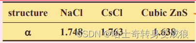
Cohesive Energy in Ionic Crystal

$$U(r)=-\frac{Na{q}^2}{4\pi {ϵ}_0^{2}r}+\frac{N{B}^{\prime }}{r^n}$$

Madelung constant: $$B^{\prime }=\sum _{j=1}^{2N-1}\frac{b}{l_j^n},\alpha =\sum _{j=1}^{2N-1}\frac{{\delta }_j}{l_j}$$

The bigger the cell, the more exactness the Madelung constant is.

1.2.3Van der Waals bond

1.2.4 Hydrogen bond

1.2.5 Covalent bond

1.2.6 Metallic bond

1.3 crystal structure and typical crystals

1.3.1 crystal structure

basic concept:

• 无定形晶体 Amorphous (Non-crystalline) Solid: All atoms have order only within a few atomic or molecular dimensions. — random arrangement in a bigger size
• 长程有序 Crystal: All atoms or molecules in the solid have a regular geometric arrangement or periodicity. — highly ordered
• 平移对称性 Periodicity: The quality of recurring at regular intervals.
• 基元 Basis: Repeatable structure units.
• 格点 Latice site: The dot representing a basis.
• 晶格 Lattice (Crystal lattice): Geometric pattern of crystal structure

Crystal Structure = Lattice + Basis

primitive vectors 基矢

position vectors 格矢

primitive unit cell 原胞

conventional unit cell 晶胞

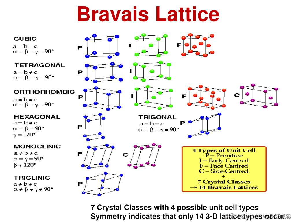
Bravais Lattice 布拉伐点阵：The geometric pattern of basis’ arrangement; all points of the lattice is identical.

Bravais lattice only summarizes the geometry of crystals, regardless of what the actual units may be.

The basis consists of the atoms, their spaces and bond angles.

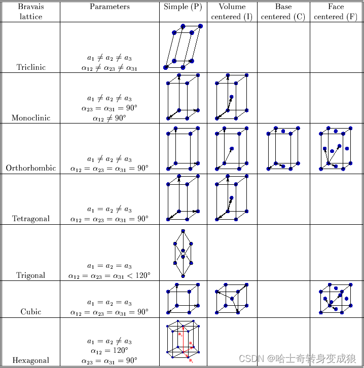
Bravais lattice:

1. Cubic 立方
2. Hexahonal 六方
3. Tetragonal 四方
4. Trigonal 三方
5. Monoclinic 单斜
6. Orthorhomic 正交
7. Triclinic 三斜

7种bravais晶系，14种bravais点阵，32点群

1.3.2 typical crystal structure

a. important parameters in crystal structure

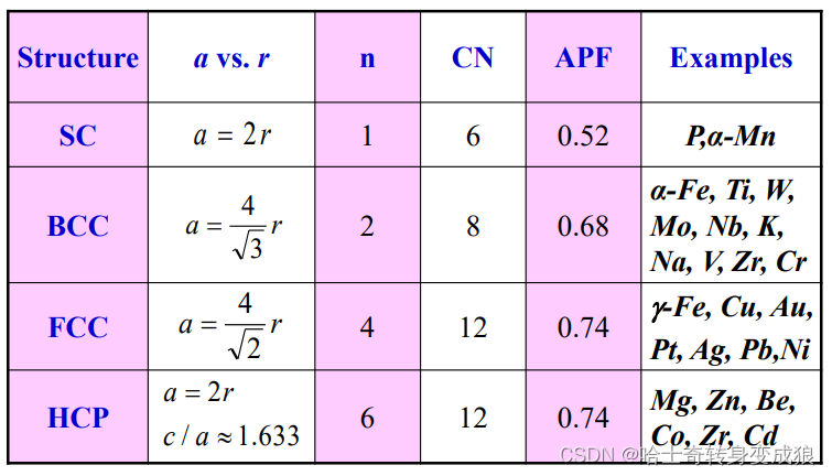
number of atoms per unit cell: n

the number of nearest neighbors, or Coordination Number: CN 配位数

Atomic Packing Factor: APF 原子堆积因数

$$APF=\frac{volumeofatomsinunitcell}{volumeofunitcell}$$

Atomic Radius: 原子半径

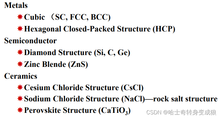
b. typical cubic structure of metal

c. typical crystal structure of semiconductor

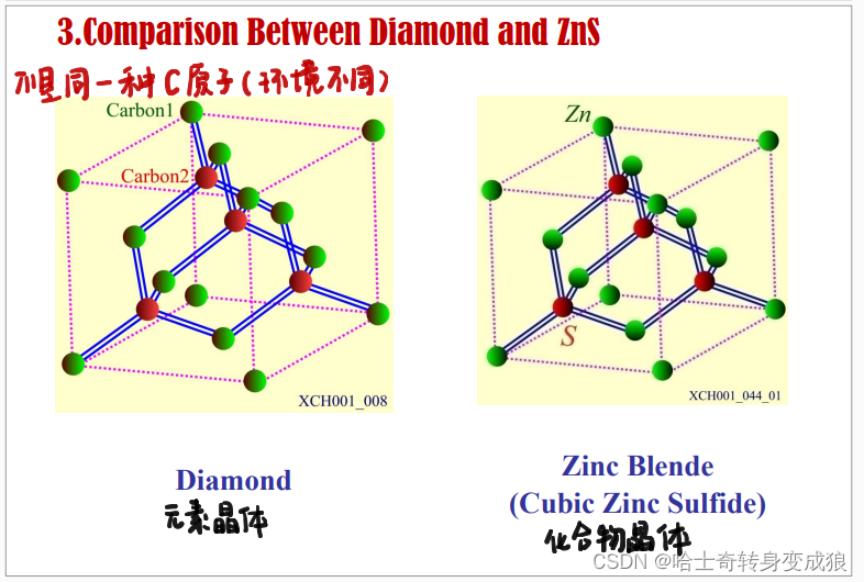
d. typical crystal structure of Ionic Crystal

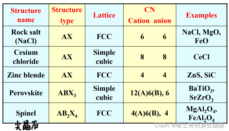
e. typical crystal structure and the Bravais Lattice

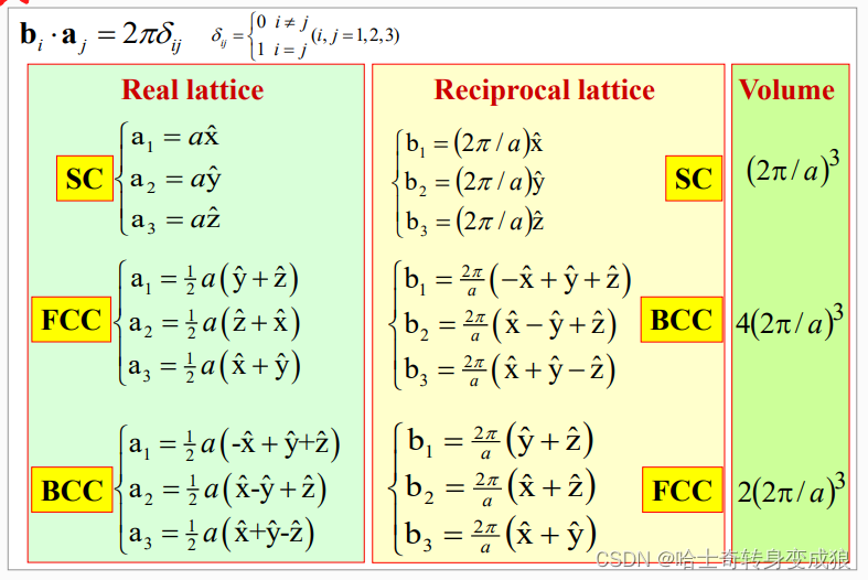
1.4 Reciprocal Lattice and Brillouin Zone

1.4.1 Reciprocal Lattice 倒易点阵

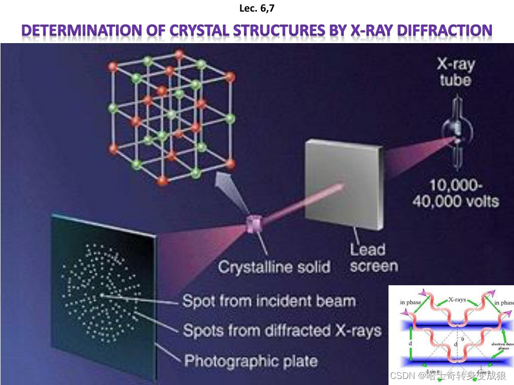
晶体衍射得到的图象（衍射斑点）是倒易点阵的二维投影空间放大。

Fourier series: 傅里叶级数
$$f(x+2\pi )=f(x)$$
$$f(x)=\frac{a_0}{2}+\sum _{n=1}^{\infty }(a_n\cos nx+b_n\sin nx)$$
$$f(x)=\sum _n{c}_n{e}^{inx},c_n=\frac{1}{2\pi }{\int }_{-\pi }^{\pi }f(x)e^{-inx}dx$$

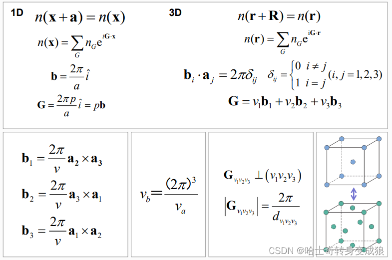
Reciprocal lattice (space): 倒易点阵，晶体空间周期性

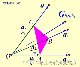
1. 如何求倒格矢？
2. 点阵和倒易点阵的原胞体积关系？
3. 正格矢和倒格矢晶面的关系？
4. 互为倒易？
   
   
   

reciprocal space & wave-vector space (k-space): 倒易空间和波矢空间（k空间）

$$u(x,t)=A\cos (\omega t-kx+{\varphi }_0)$$

$$\tilde{u}(x,t)=\tilde{A}{e}^{i(\omega t-kx)}$$

$$\mathbf{k}=\frac{2\pi }{\lambda }\hat{n},\mathbf{b}=\frac{2\pi }{a}\hat{i},\mathbf{G}=\frac{2\pi p}{a}\hat{i}$$

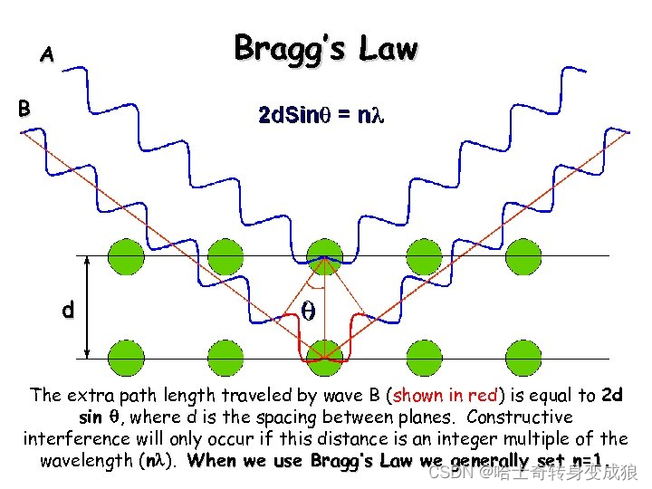
1.4.2 Crystal Diffraction 晶体衍射

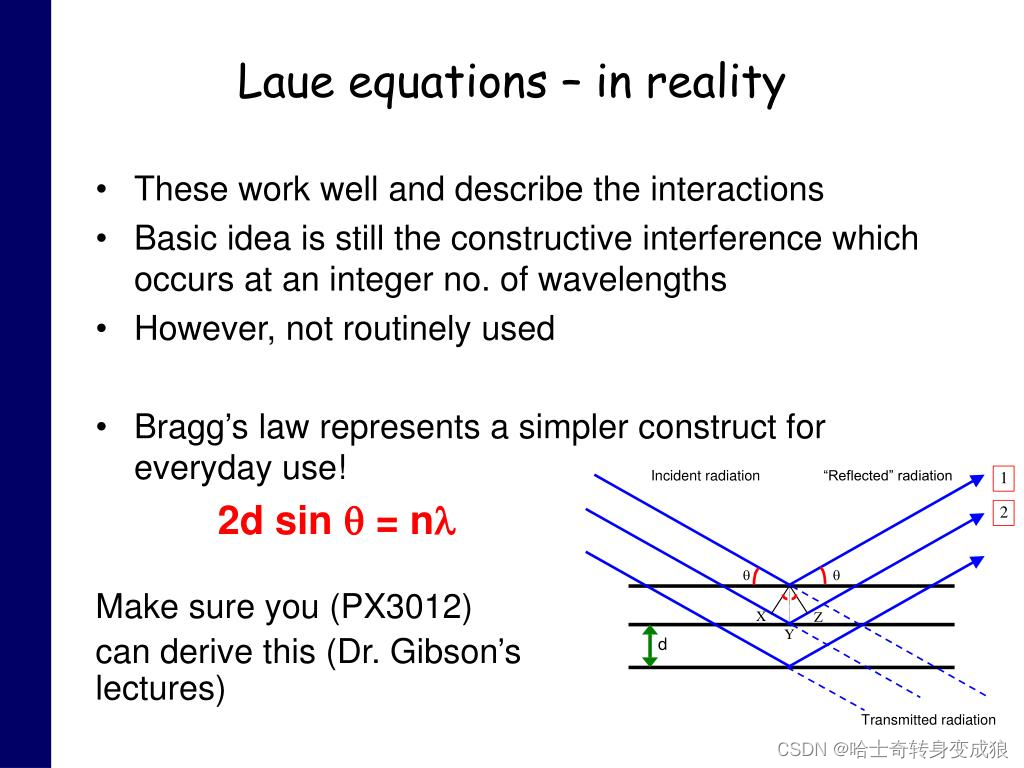
The Bragg Law：将晶体视作平行等距的晶面，将晶体对电磁波的衍射看作一组组晶面对电磁波的反射

$$2d\sin \theta =n\lambda$$

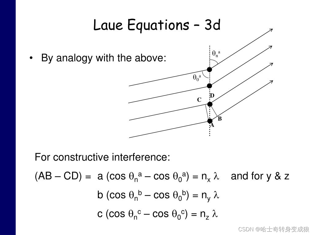
Laue equation

入射和散射的电磁波波程差：
KaTeX parse error: Undefined control sequence: \mathcf at position 35: …cos \theta ' = \̲m̲a̲t̲h̲c̲f̲{d} \cdot (\mat…$

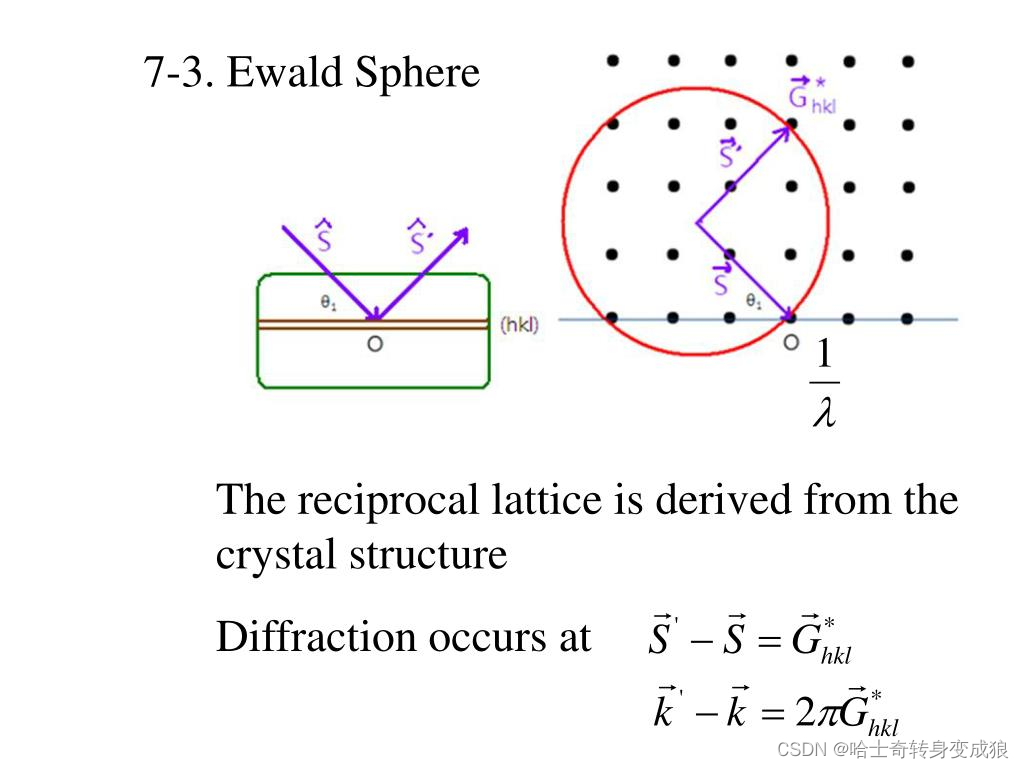
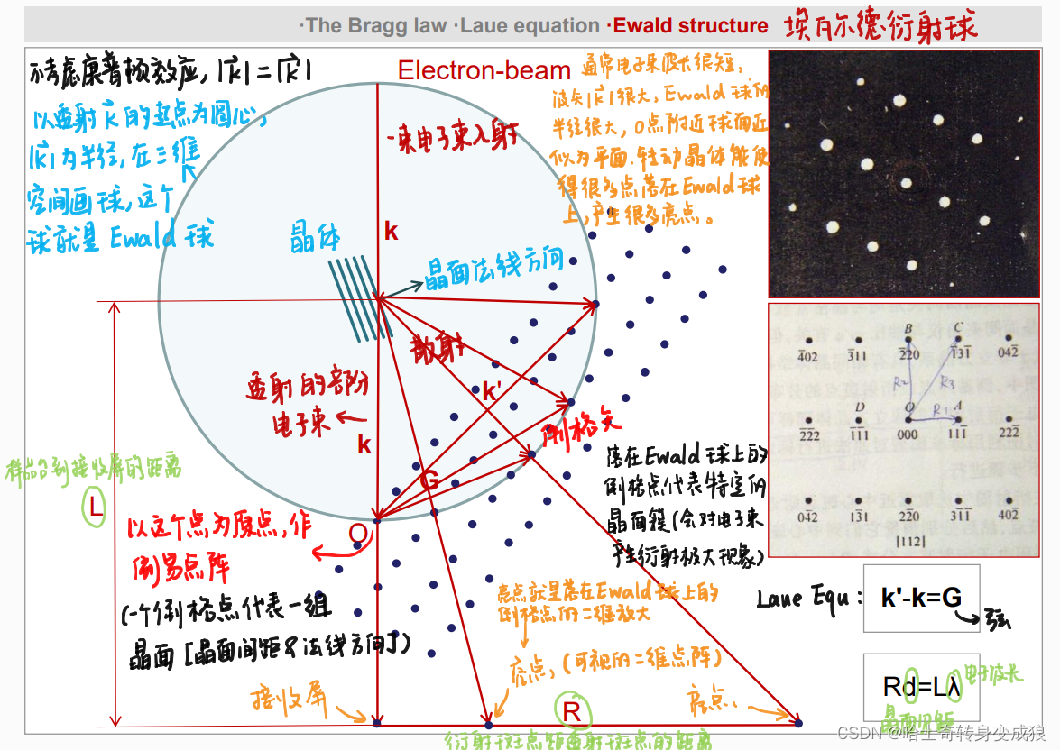
Laue Equ (与布拉格定律等价的晶体衍射关系): $${\mathbf{k}}^{\prime }-\mathbf{k}=\mathbf{G},\mathbf{\Delta k}=\mathbf{G}$$

$$2\mathbf{k}\cdot \mathbf{G}=G^2$$

Ewald structure

晶体衍射的实际过程真实存在的：电子束，样品台（晶体），接收屏上的衍射斑点。

其他的（倒易点阵、Laue Equ、Ewald球）都是虚拟的，但是它们可以帮助分析衍射的过程和原理、以及衍射斑点的位置。

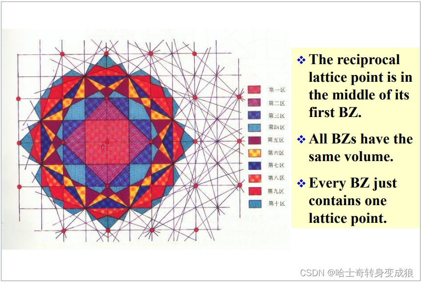
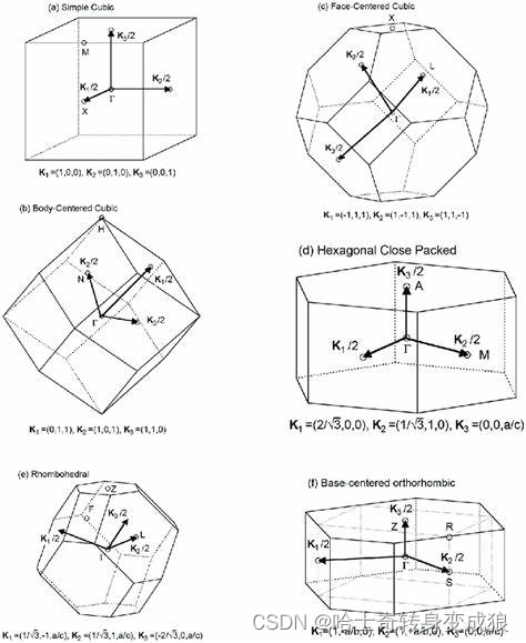
1.4.3 Brillouin Zone 布里渊区

以一个格点为原点O，找到原点O与其他格点的连线的中垂面，这些中垂面形成许多封闭区域，即布里渊区。

包围原点且最近的叫做第一布里渊区，此后称为第二、第三，以此类推。

• 倒易点阵的倒格原点在第一布里渊区的中点。
• 所有布里渊区具有相同的体积。
• 每个布里渊区含有且仅有一个格点。
• 一个布里渊区的体积等于一个原胞的体积。
• 布里渊区是晶格振动和能带理论中的常用概念。电子在跨越倒格矢中垂面（布里渊区界面）时会发生能量不连续变化。

Brillouin Zone Interface & Crystal diffraction

发生晶体衍射的条件：

1. 满足布拉格定律；
2. 满足Laue Equ.；
3. 波矢$\vec{k}$的端点落在布里渊区界面上。