本文主要是介绍【python海洋专题十】Cartopy画特定区域的地形等深线图,希望对大家解决编程问题提供一定的参考价值,需要的开发者们随着小编来一起学习吧!
【python海洋专题十】Cartopy画特定区域的地形等深线图
海洋与大气科学
前几期可以认为关于平面的元素画法🆗了
本期关于特定区域平面画法
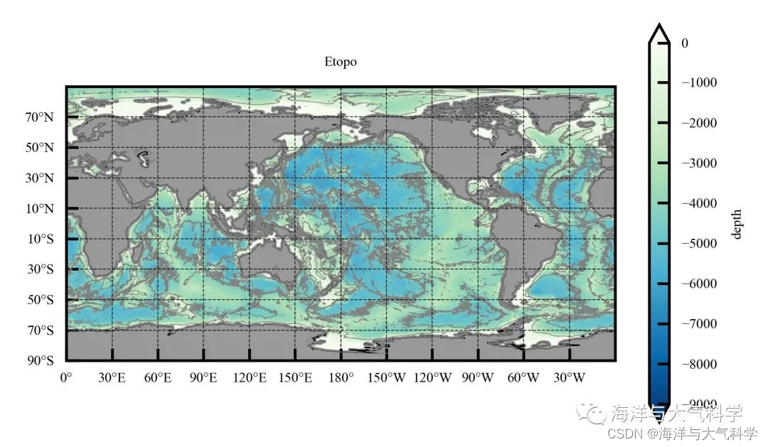
全球区域水深图
本期内容
画某元素特定区域的平面图:我有两个方法:
第一个:裁剪nc文件
第二个:掩盖其他区域,只显示特定区域的平面图。
1:裁剪nc文件
# scs's range is lon from 100 to 123;lat from 0 to 25;
print(np.where(lon >= 100))# 8400
print(np.where(lon >= 123))# 9090
print(np.where(lat >= 0))# 2700
print(np.where(lat >= 25))# 3450
lon1=lon[8400:9090]
lat1=lat[2700:3450]
ele1=ele[2700:3450,8400:9090]
目的找到范围的初始和终止位置。

大区域证明数据的裁剪!
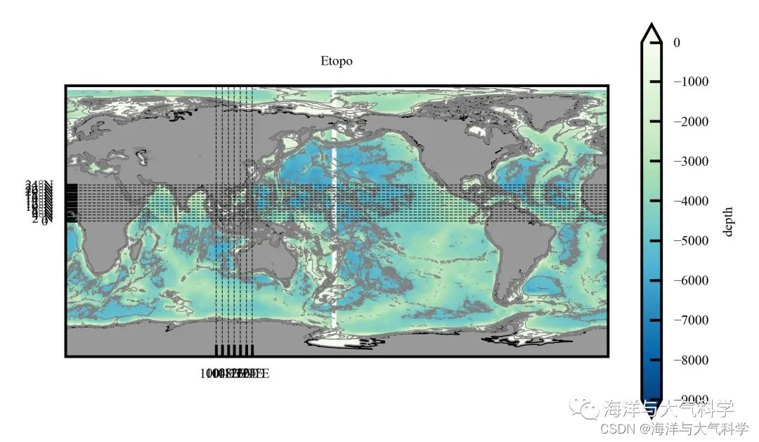
2画全球区域但只显示特定区域
ax.set_extent([100, 123, 0, 25], crs=ccrs.PlateCarree())# 设置显示范围

参考文献及其在本文中的作用
1:Python学习笔记:numpy选择符合条件数据:select、where、choose、nonzero - Hider1214 - 博客园 (cnblogs.com)
全文代码
1全球区域水深图
# -*- coding: utf-8 -*-
# %%
# Importing related function packages
import matplotlib.pyplot as plt
import cartopy.crs as ccrs
import cartopy.feature as feature
import numpy as np
import matplotlib.ticker as ticker
from cartopy import mpl
from cartopy.mpl.ticker import LongitudeFormatter, LatitudeFormatter
from cartopy.mpl.gridliner import LONGITUDE_FORMATTER, LATITUDE_FORMATTER
from matplotlib.font_manager import FontProperties
from netCDF4 import Dataset
from palettable.cmocean.diverging import Delta_4
from palettable.colorbrewer.sequential import GnBu_9
from palettable.colorbrewer.sequential import Blues_9
from palettable.scientific.diverging import Roma_20
from pylab import *
def reverse_colourmap(cmap, name='my_cmap_r'):reverse = []k = []for key in cmap._segmentdata:k.append(key)channel = cmap._segmentdata[key]data = []for t in channel:data.append((1 - t[0], t[2], t[1]))reverse.append(sorted(data))LinearL = dict(zip(k, reverse))my_cmap_r = mpl.colors.LinearSegmentedColormap(name, LinearL)return my_cmap_rcmap = Blues_9.mpl_colormap
cmap_r = reverse_colourmap(cmap)
cmap1 = GnBu_9.mpl_colormap
cmap_r1 = reverse_colourmap(cmap1)
cmap2 = Roma_20.mpl_colormap
cmap_r2 = reverse_colourmap(cmap2)
# read data
a = Dataset('D:\pycharm_work\data\etopo2.nc')
print(a)
lon = a.variables['lon'][:]
lat = a.variables['lat'][:]
ele = a.variables['topo'][:,:]
lon1=lon[1:10800:110]
lat1=lat[1:5400:110]
ele1=ele[1:5400:110,1:10800:110]
print(len(lon1))
print(len(lat))
# 图三
# 设置地图全局属性
scale = '50m'
plt.rcParams['font.sans-serif'] = ['Times New Roman']  # 设置整体的字体为Times New Roman
fig = plt.figure(dpi=300, figsize=(3, 2), facecolor='w', edgecolor='blue')#设置一个画板,将其返还给fig
ax = fig.add_axes([0.05, 0.08, 0.92, 0.8], projection=ccrs.PlateCarree(central_longitude=180))
ax.set_extent([0, 360, -90, 90], crs=ccrs.PlateCarree())# 设置显示范围
land = feature.NaturalEarthFeature('physical', 'land', scale, edgecolor='face',facecolor=feature.COLORS['land'])
ax.add_feature(land, facecolor='0.6')
ax.add_feature(feature.COASTLINE.with_scale('50m'), lw=0.3)#添加海岸线:关键字lw设置线宽;linestyle设置线型
cs = ax.contourf(lon1, lat1, ele1, levels=np.arange(-9000,0,20),extend='both',cmap=cmap_r1, transform=ccrs.PlateCarree())
# ------colorbar设置
cb = plt.colorbar(cs, ax=ax, extend='both', orientation='vertical',ticks=np.linspace(-9000, 0, 10))
cb.set_label('depth', fontsize=4, color='k')#设置colorbar的标签字体及其大小
cb.ax.tick_params(labelsize=4, direction='in') #设置colorbar刻度字体大小。
cf = ax.contour(lon, lat, ele[:, :], levels=np.linspace(-9000, 0, 5),colors='gray', linestyles='-',linewidths=0.2,transform=ccrs.PlateCarree())
# 添加标题
ax.set_title('Etopo', fontsize=4)
# 利用Formatter格式化刻度标签
ax.set_xticks(np.arange(0, 360, 30), crs=ccrs.PlateCarree())#添加经纬度
ax.set_xticklabels(np.arange(0, 360, 30), fontsize=4)
ax.set_yticks(np.arange(-90, 90, 20), crs=ccrs.PlateCarree())
ax.set_yticklabels(np.arange(-90, 90, 20), fontsize=4)
ax.xaxis.set_major_formatter(LongitudeFormatter())
ax.yaxis.set_major_formatter(LatitudeFormatter())
ax.tick_params(color='k', direction='in')#更改刻度指向为朝内,颜色设置为蓝色
gl = ax.gridlines(crs=ccrs.PlateCarree(), draw_labels=False, xlocs=np.arange(-180, 180, 30), ylocs=np.arange(-90, 90, 20),linewidth=0.25, linestyle='--', color='k', alpha=0.8)#添加网格线
gl.top_labels, gl.bottom_labels, gl.right_labels, gl.left_labels = False, False, False, False
plt.savefig('scs_elevation03.jpg', dpi=600, bbox_inches='tight', pad_inches=0.1)  # 输出地图,并设置边框空白紧密
plt.show()
2:裁剪nc文件;
# -*- coding: utf-8 -*-
# %%
# Importing related function packages
import matplotlib.pyplot as plt
import cartopy.crs as ccrs
import cartopy.feature as feature
import numpy as np
import matplotlib.ticker as ticker
from cartopy import mpl
from cartopy.mpl.ticker import LongitudeFormatter, LatitudeFormatter
from cartopy.mpl.gridliner import LONGITUDE_FORMATTER, LATITUDE_FORMATTER
from matplotlib.font_manager import FontProperties
from netCDF4 import Dataset
from palettable.cmocean.diverging import Delta_4
from palettable.colorbrewer.sequential import GnBu_9
from palettable.colorbrewer.sequential import Blues_9
from palettable.scientific.diverging import Roma_20
from pylab import *
def reverse_colourmap(cmap, name='my_cmap_r'):reverse = []k = []for key in cmap._segmentdata:k.append(key)channel = cmap._segmentdata[key]data = []for t in channel:data.append((1 - t[0], t[2], t[1]))reverse.append(sorted(data))LinearL = dict(zip(k, reverse))my_cmap_r = mpl.colors.LinearSegmentedColormap(name, LinearL)return my_cmap_rcmap = Blues_9.mpl_colormap
cmap_r = reverse_colourmap(cmap)
cmap1 = GnBu_9.mpl_colormap
cmap_r1 = reverse_colourmap(cmap1)
cmap2 = Roma_20.mpl_colormap
cmap_r2 = reverse_colourmap(cmap2)
# read data
a = Dataset('D:\pycharm_work\data\etopo2.nc')
print(a)
lon = a.variables['lon'][:]
lat = a.variables['lat'][:]
ele = a.variables['topo'][:]
print(lon)
print(lat)
# scs's range is lon from 100 to 123;lat from 0 to 25;
# so
print(np.where(lon >= 100))# 8400
print(np.where(lon >= 123))# 9090
print(np.where(lat >= 0))# 2700
print(np.where(lat >= 25))# 3450
lon1=lon[8400:9090]
lat1=lat[2700:3450]
ele1=ele[2700:3450,8400:9090]
# 图三
# 设置地图全局属性
scale = '50m'
plt.rcParams['font.sans-serif'] = ['Times New Roman']  # 设置整体的字体为Times New Roman
fig = plt.figure(dpi=300, figsize=(3, 2), facecolor='w', edgecolor='blue')#设置一个画板,将其返还给fig
ax = fig.add_axes([0.05, 0.08, 0.92, 0.8], projection=ccrs.PlateCarree(central_longitude=180))
ax.set_extent([100, 123, 0, 25], crs=ccrs.PlateCarree())# 设置显示范围
land = feature.NaturalEarthFeature('physical', 'land', scale, edgecolor='face',facecolor=feature.COLORS['land'])
ax.add_feature(land, facecolor='0.6')
ax.add_feature(feature.COASTLINE.with_scale('50m'), lw=0.3)#添加海岸线:关键字lw设置线宽;linestyle设置线型
cs = ax.contourf(lon1, lat1, ele1, levels=np.arange(-9000,0,20),extend='both',cmap=cmap_r1, transform=ccrs.PlateCarree())
# ------colorbar设置
cb = plt.colorbar(cs, ax=ax, extend='both', orientation='vertical',ticks=np.linspace(-9000, 0, 10))
cb.set_label('depth', fontsize=4, color='k')#设置colorbar的标签字体及其大小
cb.ax.tick_params(labelsize=4, direction='in') #设置colorbar刻度字体大小。
cf = ax.contour(lon, lat, ele[:, :], levels=[-5000,-2000,-500,-300,-100,-50,-10],colors='gray', linestyles='-',linewidths=0.2,transform=ccrs.PlateCarree())
# 添加标题
ax.set_title('Etopo', fontsize=4)
# 利用Formatter格式化刻度标签
ax.set_xticks(np.arange(100, 123, 4), crs=ccrs.PlateCarree())#添加经纬度
ax.set_xticklabels(np.arange(100, 123, 4), fontsize=4)
ax.set_yticks(np.arange(0, 25, 2), crs=ccrs.PlateCarree())
ax.set_yticklabels(np.arange(0, 25, 2), fontsize=4)
ax.xaxis.set_major_formatter(LongitudeFormatter())
ax.yaxis.set_major_formatter(LatitudeFormatter())
ax.tick_params(color='k', direction='in')#更改刻度指向为朝内,颜色设置为蓝色
gl = ax.gridlines(crs=ccrs.PlateCarree(), draw_labels=False, xlocs=np.arange(100, 123, 4), ylocs=np.arange(0, 25, 2),linewidth=0.25, linestyle='--', color='k', alpha=0.8)#添加网格线
gl.top_labels, gl.bottom_labels, gl.right_labels, gl.left_labels = False, False, False, False
plt.savefig('scs_elevation1.jpg', dpi=600, bbox_inches='tight', pad_inches=0.1)  # 输出地图,并设置边框空白紧密
plt.show()
3:掩盖其他区域,只显示特定区域的平面图。
# -*- coding: utf-8 -*-
# %%
# Importing related function packages
import matplotlib.pyplot as plt
import cartopy.crs as ccrs
import cartopy.feature as feature
import numpy as np
import matplotlib.ticker as ticker
from cartopy import mpl
from cartopy.mpl.ticker import LongitudeFormatter, LatitudeFormatter
from cartopy.mpl.gridliner import LONGITUDE_FORMATTER, LATITUDE_FORMATTER
from matplotlib.font_manager import FontProperties
from netCDF4 import Dataset
from palettable.cmocean.diverging import Delta_4
from palettable.colorbrewer.sequential import GnBu_9
from palettable.colorbrewer.sequential import Blues_9
from palettable.scientific.diverging import Roma_20
from pylab import *
def reverse_colourmap(cmap, name='my_cmap_r'):reverse = []k = []for key in cmap._segmentdata:k.append(key)channel = cmap._segmentdata[key]data = []for t in channel:data.append((1 - t[0], t[2], t[1]))reverse.append(sorted(data))LinearL = dict(zip(k, reverse))my_cmap_r = mpl.colors.LinearSegmentedColormap(name, LinearL)return my_cmap_rcmap = Blues_9.mpl_colormap
cmap_r = reverse_colourmap(cmap)
cmap1 = GnBu_9.mpl_colormap
cmap_r1 = reverse_colourmap(cmap1)
cmap2 = Roma_20.mpl_colormap
cmap_r2 = reverse_colourmap(cmap2)
# read data
a = Dataset('D:\pycharm_work\data\etopo2.nc')
print(a)
lon = a.variables['lon'][:]
lat = a.variables['lat'][:]
ele = a.variables['topo'][:,:]
lon1=lon[1:10800:110]
lat1=lat[1:5400:110]
ele1=ele[1:5400:110,1:10800:110]
print(len(lon1))
print(len(lat))
# 图三
# 设置地图全局属性
scale = '50m'
plt.rcParams['font.sans-serif'] = ['Times New Roman']  # 设置整体的字体为Times New Roman
fig = plt.figure(dpi=300, figsize=(3, 2), facecolor='w', edgecolor='blue')#设置一个画板,将其返还给fig
ax = fig.add_axes([0.05, 0.08, 0.92, 0.8], projection=ccrs.PlateCarree(central_longitude=180))
ax.set_extent([100, 123, 0, 25], crs=ccrs.PlateCarree())# 设置显示范围
land = feature.NaturalEarthFeature('physical', 'land', scale, edgecolor='face',facecolor=feature.COLORS['land'])
ax.add_feature(land, facecolor='0.6')
ax.add_feature(feature.COASTLINE.with_scale('50m'), lw=0.3)#添加海岸线:关键字lw设置线宽;linestyle设置线型
cs = ax.contourf(lon1, lat1, ele1, levels=np.arange(-9000,0,20),extend='both',cmap=cmap_r1, transform=ccrs.PlateCarree())
# ------colorbar设置
cb = plt.colorbar(cs, ax=ax, extend='both', orientation='vertical',ticks=np.linspace(-9000, 0, 10))
cb.set_label('depth', fontsize=4, color='k')#设置colorbar的标签字体及其大小
cb.ax.tick_params(labelsize=4, direction='in') #设置colorbar刻度字体大小。
cf = ax.contour(lon, lat, ele[:, :], levels=np.linspace(-9000, 0, 5),colors='gray', linestyles='-',linewidths=0.2,transform=ccrs.PlateCarree())
# 添加标题
ax.set_title('Etopo', fontsize=4)
# 利用Formatter格式化刻度标签
ax.set_xticks(np.arange(100, 123, 5), crs=ccrs.PlateCarree())#添加经纬度
ax.set_xticklabels(np.arange(100, 123, 5), fontsize=4)
ax.set_yticks(np.arange(0, 25, 5), crs=ccrs.PlateCarree())
ax.set_yticklabels(np.arange(0, 25, 5), fontsize=4)
ax.xaxis.set_major_formatter(LongitudeFormatter())
ax.yaxis.set_major_formatter(LatitudeFormatter())
ax.tick_params(color='k', direction='in')#更改刻度指向为朝内,颜色设置为蓝色
gl = ax.gridlines(crs=ccrs.PlateCarree(), draw_labels=False, xlocs=np.arange(100, 123, 5), ylocs=np.arange(0, 25, 5),linewidth=0.25, linestyle='--', color='k', alpha=0.8)#添加网格线
gl.top_labels, gl.bottom_labels, gl.right_labels, gl.left_labels = False, False, False, False
plt.savefig('scs_elevation03.jpg', dpi=600, bbox_inches='tight', pad_inches=0.1)  # 输出地图,并设置边框空白紧密
plt.show()
这篇关于【python海洋专题十】Cartopy画特定区域的地形等深线图的文章就介绍到这儿,希望我们推荐的文章对编程师们有所帮助!


