本文主要是介绍美国King County房价训练赛分析流程,希望对大家解决编程问题提供一定的参考价值,需要的开发者们随着小编来一起学习吧!
花了一点时间做了下这个比赛,当作是数据分析的练手项目了。
比赛详细信息及数据下载
导入一些必要的库
import pandas as pd
import matplotlib.pyplot as plt
import seaborn as sns
import numpy as np
1. 数据清洗
1.1 添加名称,分离变量
def get_feature(df):sell_year, sell_month, sell_day, build_age, repair_age = [], [], [], [], []for [time, build_year, repair_year] in df[['Time', 'YearOfBuild', 'YearOfRepair']].values:#将销售时间转化为销售年份、销售月份、销售日期四个变量year, month, day = int(str(time)[0:4]), int(str(time)[4:6]), int(str(time)[6:8])sell_year.append(year)sell_month.append(month)sell_day.append(day)#将建造/修复年份分别转化为当售出时build_age.append(year-build_year)if repair_year == 0:repair_age.append(0)else:repair_age.append(year-repair_year)    df['sell_year'] = sell_yeardf['sell_month'] = sell_monthdf['sell_day'] = sell_daydf['build_age'] = build_agedf['repair_age'] = repair_age#根据房价 加权出理想中心点,Distance变量即为与中心点的“经纬度距离”lon = np.average(df_train['Longitude'],weights=df_price['Price']/df_train['AreaOfHouse'])lat = np.average(df_train['Latitude'],weights=df_price['Price']/df_train['AreaOfHouse'])df['Distance'] = np.power(lon-df['Longitude'],2)+np.power(lat-df['Latitude'],2)df.drop(columns=['Time'], inplace=True)
columns = ['Time', 'NumOfBeedroom', 'NumOfBathroom', 'AreaOfHouse', 'AreaOfParking', 'NumOfFloor', 'Rating', 'AreaOfBuilding','AreaOfUnderGround', 'YearOfBuild', 'YearOfRepair', 'Latitude','Longitude']
df_train = pd.read_csv('kc_train.csv', header=None)
df_test = pd.read_csv('kc_test.csv', header=None)
# 添加列名
df_price = pd.DataFrame(columns=['Price'])
df_price['Price'] = df_train[1]
df_train.drop(columns=[1], inplace=True)
df_train.columns, df_test.columns = columns, columns
# 处理变量
get_feature(df_train)
get_feature(df_test)
# 落地特征工程后的数据集
df_train.to_csv('data/train_1.csv', index=False)
df_price.to_csv('data/label_1.csv', index=False)
df_test.to_csv('data/test_1.csv', index=False)
print('数据集已存储于data。')
数据集已存储于data。
1.2 空值处理
df = pd.concat([pd.read_csv('data/train_1.csv'),pd.read_csv('data/label_1.csv')],axis=1)
print(df.info())
<class 'pandas.core.frame.DataFrame'>
RangeIndex: 10000 entries, 0 to 9999
Data columns (total 19 columns):
NumOfBeedroom        10000 non-null int64
NumOfBathroom        10000 non-null float64
AreaOfHouse          10000 non-null int64
AreaOfParking        10000 non-null int64
NumOfFloor           10000 non-null float64
Rating               10000 non-null int64
AreaOfBuilding       10000 non-null int64
AreaOfUnderGround    10000 non-null int64
YearOfBuild          10000 non-null int64
YearOfRepair         10000 non-null int64
Latitude             10000 non-null float64
Longitude            10000 non-null float64
sell_year            10000 non-null int64
sell_month           10000 non-null int64
sell_day             10000 non-null int64
build_age            10000 non-null int64
repair_age           10000 non-null int64
Distance             10000 non-null float64
Price                10000 non-null int64
dtypes: float64(5), int64(14)
memory usage: 1.4 MB
None
我们可以看到数据集的14列计数均为10000,不存在空值。
若存在空值,则采用删去该条数据或插值的方法。
数值类型为常见的整数和浮点数,不存在日期和文本类型。
2. 数据观察
2.1 数据概览
简便方法是通过pandas_profiling
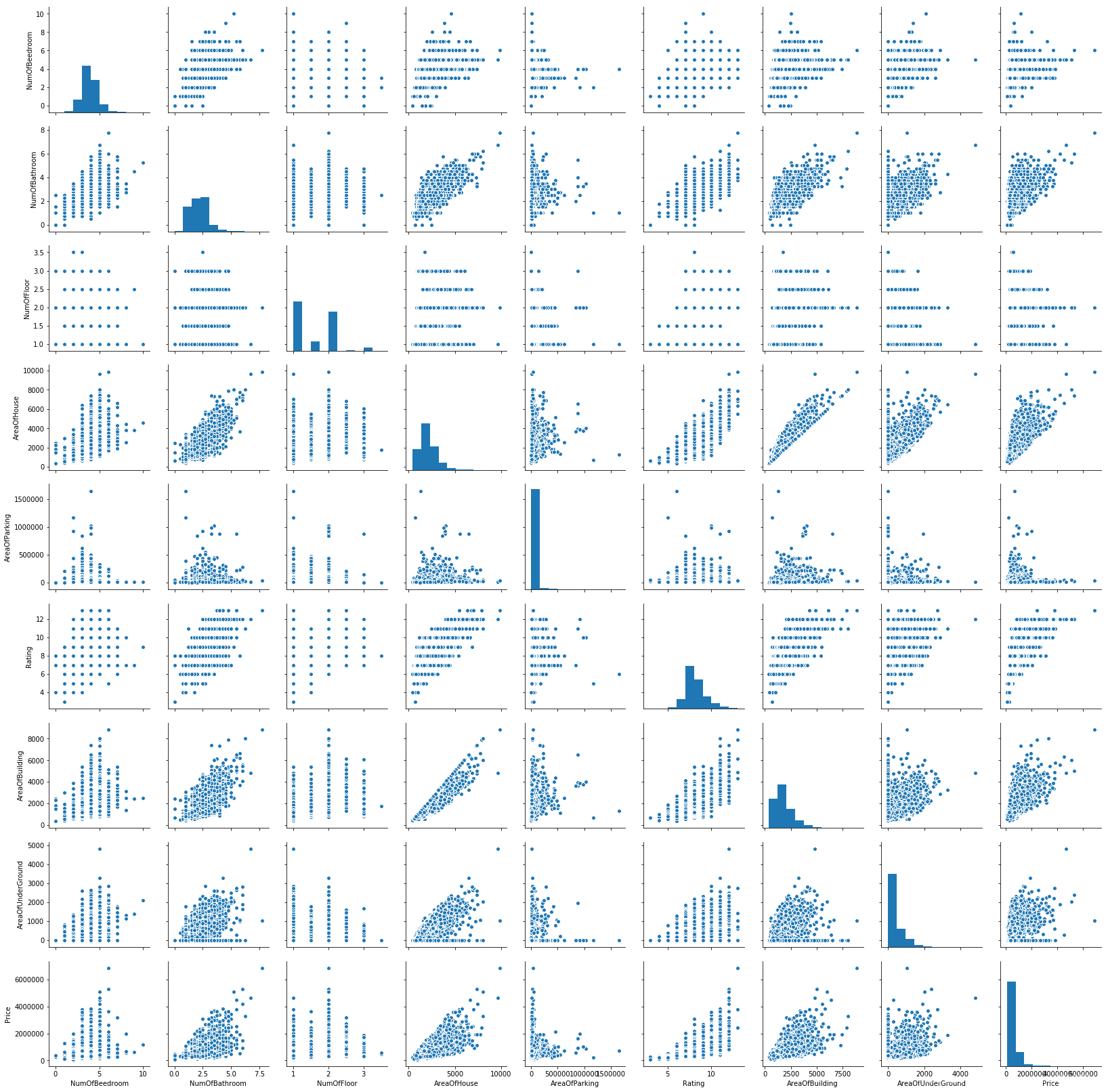
或者通过sns.pairplot 观察某些变量的分布情况
import pandas_profiling
df = pd.concat([pd.read_csv('data/train_1.csv'),pd.read_csv('data/label_1.csv')],axis=1)
#pandas_profiling.ProfileReport(df)
profile = df.profile_report(title="Census Dataset")
profile.to_file(output_file="census_report.html")
df = pd.concat([pd.read_csv('data/train_1.csv'),pd.read_csv('data/label_1.csv')],axis=1)
col =[ 'NumOfBeedroom', 'NumOfBathroom', 'NumOfFloor', 'AreaOfHouse','AreaOfParking',  'Rating', 'AreaOfBuilding', 'AreaOfUnderGround',  'Price']
sns.pairplot(df[col])
plt.show()
2.2 相关性分析
df = pd.concat([pd.read_csv('data/train_1.csv'),pd.read_csv('data/label_1.csv')],axis=1)
plt.subplots(figsize=(12,9))
corrmat = df.corr()
sns.heatmap(corrmat, vmax=0.9, square=True,center=0,cmap='Reds_r')
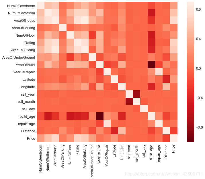
直接做热力图比较乱,选择和销售价格相关性最好的十个变量做热力图。
df = pd.concat([pd.read_csv('data/train_1.csv'),pd.read_csv('data/label_1.csv')],axis=1)
plt.figure(figsize=(12,9))
cols = df.corr().nlargest(10, 'Price')['Price'].index
cm = np.corrcoef(df[cols].values.T)
sns.set(font_scale=1.25)
hm = sns.heatmap(cm, cbar=True, annot=True, square=True, fmt='.2f', annot_kws={'size': 10}, yticklabels=cols.values, xticklabels=cols.values)
plt.show()
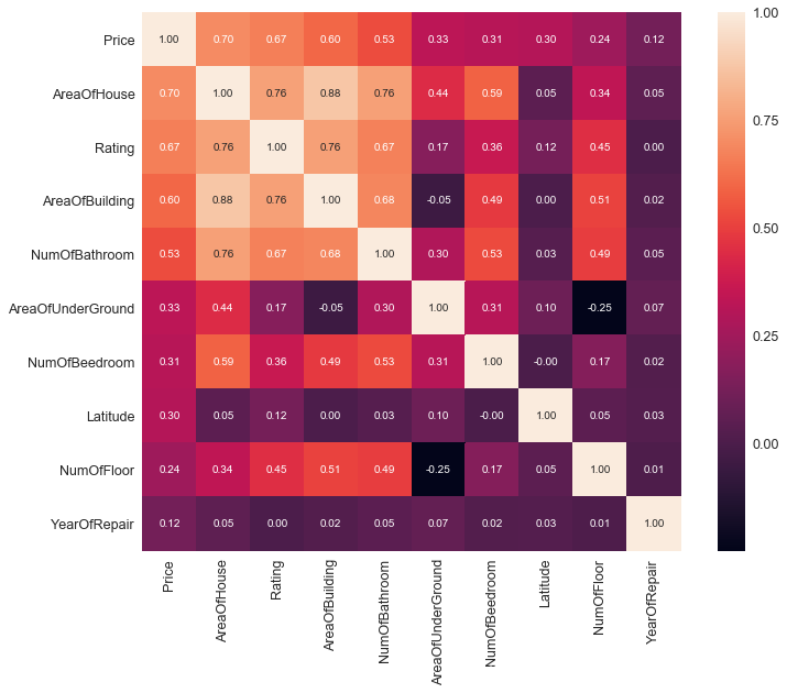
我们看到和销售价格相关性最好的为房屋面积,房屋评分,建筑面积,地下室面积,浴室和卧室的数量。
若数据量较大时,可仅选择相关性较好的参数用于后续模型分析。
以销售价格和房屋面积,结合房屋评分为例,我们进一步分析其相关性。
df = pd.concat([pd.read_csv('data/train_1.csv'),pd.read_csv('data/label_1.csv')],axis=1)
%matplotlib inline
plt.subplots(figsize=(12,9))
sns.boxplot(x='Rating',y='Price',data=df)
plt.show()
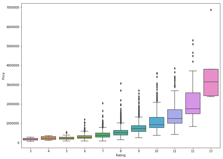
显而易见的是,评分越高的房屋销售价格越高,并且评分较高的房屋销售价格容易出现异常高值。
定义 房价 = 销售价格 / 房屋面积
观察
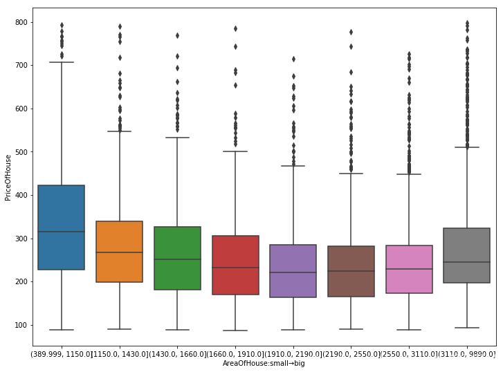
df = pd.concat([pd.read_csv('data/train_1.csv'),pd.read_csv('data/label_1.csv')],axis=1)
df['PriceOfHouse'] = df['Price']/df['AreaOfHouse']
df['qcut'] = pd.qcut(df['AreaOfHouse'],8)
plt.subplots(figsize=(12,9))
sns.boxplot('qcut','PriceOfHouse',data=df)
x = plt.xticks()
plt.xlabel('AreaOfHouse:small→big')
plt.show()
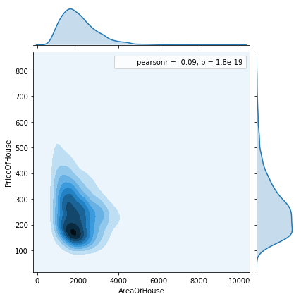
%matplotlib inline
df = pd.concat([pd.read_csv('data/train_1.csv'),pd.read_csv('data/label_1.csv')],axis=1)
df['PriceOfHouse'] = df['Price']/df['AreaOfHouse']
sns.jointplot('AreaOfHouse','PriceOfHouse',data=df,kind='kde')
plt.show()
把数据按房屋面积从小到大平均分成八份后,发现一些直接做散点图不能看到的现象。
总的来说,房价随房屋面积的增加而逐渐降低(r=-0.09,p<0.01),但是在房屋面积非常大时,房价出现了回升
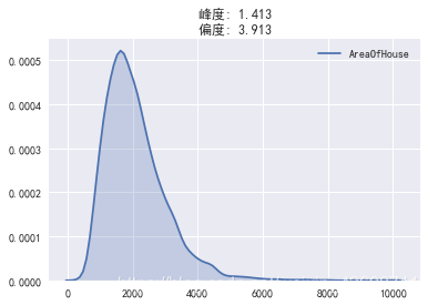
2.3 分布分析
以AreaOfHouse(房屋面积)为例
我们发现该变量为正偏态分布,而且峰度较高。为了在模型中避免因为偏度问题带来的误差,需要对数据做一些变化。
将数组取对数后(备用方法:开根号,倒数等),峰度和偏度大幅接近正态分布的值
%matplotlib inline
plt.rcParams['font.sans-serif'] = ['SimHei']  # 用来正常显示中文标签
plt.rcParams['axes.unicode_minus'] = False  # 用来正常显示负号
def view_data(df_series):fig = plt.figure()sns.kdeplot(df_series,shade=True)text = '峰度: ' + str(np.round(df_series.skew(),3)) +'\n偏度: ' +str(np.round(df_series.kurt(),3))plt.title(text)
df = pd.concat([pd.read_csv('data/train_1.csv'),pd.read_csv('data/label_1.csv')],axis=1)
view_data(df['AreaOfHouse'])
df = pd.concat([pd.read_csv('data/train_1.csv'),pd.read_csv('data/label_1.csv')],axis=1)
view_data(np.log(df['AreaOfHouse']))
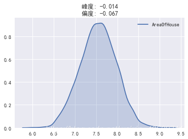
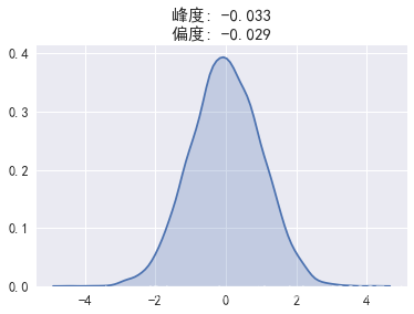
print('附:正态分布数组的偏度与峰度')
view_data(pd.Series(np.random.randn(10000)))
附:正态分布数组的偏度与峰度
2.4 主成分分析
当数据集列数过多时,除了剔除明显不相关的变量,我们可以用主成分分析将数据降维,以减少模型运算量。
from sklearn.decomposition import PCA
df = pd.concat([pd.read_csv('data/train_1.csv'),pd.read_csv('data/label_1.csv')],axis=1)
model = PCA(n_components=5)
model.fit_transform(df)
exp_var = np.round(model.explained_variance_ratio_,decimals=5)
print('各个主成分解释的方差百分比',exp_var)
各个主成分解释的方差百分比 [9.8528e-01 1.4710e-02 1.0000e-05 0.0000e+00 0.0000e+00]
主成分1和2几乎解释了全部的方差。
因此,若数据量过于庞大,可用主成分1和主成分2输入模型运算。
3. 模型选择
3.1 线性回归
此外也可通过itertools.combinations函数(%load(run) 增加参数.py),实现变量排列组合的线性回归,为了更好的结果(更小的测试集标准误差)
df_train = pd.read_csv('data/train_1.csv')
y_train = pd.read_csv('data/label_1.csv').values
df_test = pd.read_csv('data/test_1.csv')
# 归一化变量(对训练集和测试集统一归一化)
def normlized(df,maxmin):for item in df.columns:df[item] = (df[item] - maxmin[item]['min'] )/(maxmin[item]['max'] -maxmin[item]['min'] )
maxmin = df_train.append(df_test).describe()
normlized(df_train,maxmin)
normlized(df_test,maxmin)
from sklearn.linear_model import LinearRegression
from sklearn.cross_validation import train_test_split
X_train,X_test,Y_train,Y_test = train_test_split(df_train,y_train,train_size=.7)
model = LinearRegression()
model.fit(X_train,Y_train)
print('测试集的标准误差为%.2f' %np.std(model.predict(X_test)-Y_test))
print('测试集的模型得分为%.2f' %model.score(X_test,Y_test))
df_output = pd.DataFrame(data=model.predict(df_test),columns=['price'])
df_output.to_csv('result.csv',index=False, encoding='utf-8')
测试集的标准误差为220881.87
测试集的模型得分为0.67
3.2 其他模型
from sklearn.linear_model import Ridge,Lasso
from sklearn import tree,svm,neighbors,ensemble
# 线性回归   std=226038#排名458
model = LinearRegression()
# 岭回归
model = Ridge()
# 岭回归
model = Lasso()
# 决策树 score= 0.74 std= 225830  ['房屋面积', '房屋评分', '建筑年份']
model = tree.DecisionTreeRegressor()
# 支持向量机回归
model = svm.SVR()
# K邻近回归 score= 0.7635649915125772 std= 325610.9279272832  ['楼层数', '房屋评分', '修复年份', '纬度', '经度']
model = neighbors.KNeighborsRegressor()
# 随机森林回归
model = ensemble.RandomForestRegressor(n_estimators=20)
# Adaboost 回归
model = ensemble.AdaBoostRegressor(n_estimators=50)
# 梯度增强随机森林回归
model = ensemble.GradientBoostingRegressor(n_estimators=100)
# Bagging回归
model = ensemble.BaggingRegressor()
# ExtraTree 回归
model = tree.ExtraTreeRegressor
3.3 神经网络-Sequential 序贯模型
import pandas as pd
import numpy as np
from keras.layers import Dense,Dropout
from keras.models import Sequential
from sklearn.model_selection import train_test_split
from keras import metrics
df_train = pd.read_csv('data/train_1.csv')
y_train = pd.read_csv('data/label_1.csv').values
df_test = pd.read_csv('data/test_1.csv')
# 归一化变量(对训练集和测试集统一归一化)
def normlized(df,maxmin):for item in df.columns:df[item] = (df[item] - maxmin[item]['min'] )/(maxmin[item]['max'] -maxmin[item]['min'] )maxmin = df_train.append(df_test).describe()
normlized(df_train,maxmin)
normlized(df_test,maxmin)
#Dense 全连接层 Activation 激活层 Dropout 防止过拟合
model = Sequential([Dense(units=90, activation='relu', input_shape=(len(df_train.columns), )),Dropout(0.5),Dense(units=45, activation='relu'),Dropout(0.5),Dense(units=30,activation='relu'),Dropout(0.25),Dense(units=15, activation='relu'),Dropout(0.1),Dense(units=1,activation=None)# 此处不能使用激活函数,因为放假是放射的])# 官网使用mse计算损失
model.compile(loss='mean_squared_error',optimizer='adam',metrics=[metrics.mae])
model.summary()x_tra, x_val, y_tra, y_val = train_test_split(df_train, y_train, test_size=0.3, random_state=2019)
history = model.fit(x_tra, y_tra, batch_size=64, epochs=50, verbose=1, validation_data=(x_val, y_val),)#损失函数画图
import matplotlib.pyplot as plt
plt.plot(np.arange(len(history.history['loss'])), history.history['loss'], label='train')
plt.plot(np.arange(len(history.history['val_loss'])), history.history['val_loss'], label='valid')
plt.xlabel('epochs')
plt.ylabel('losses')
plt.legend(loc=0)
plt.show()result = pd.DataFrame({'price': model.predict(df_test).reshape(1, -1)[0]})
result.to_csv('result.csv', index=False, encoding='utf-8')
尾言

最终神经网络结果的排名还是较线性回归和其他模型更好一些,#312(总队伍数1761,提交结果5678),并不是很好的成绩,但是提升的方法无非对多加几层神经网络或是对不同模型的结果加权平均。一味地追求排名可能有点浪费时间,对整个数据分析流程的理解和掌握可能是更重要的。
这篇关于美国King County房价训练赛分析流程的文章就介绍到这儿,希望我们推荐的文章对编程师们有所帮助!


