Python 画雷达反射率图

1. 导库

import numpy as np
from matplotlib import pyplot as plt
from matplotlib.cm import get_cmap
from matplotlib.colors import from_levels_and_colors
import cartopy.crs as ccrs
import cartopy.io.shapereader as shpreader
from cartopy.feature import NaturalEarthFeature, COLORS
from netCDF4 import Dataset
from wrf import (getvar, to_np, get_cartopy, latlon_coords, vertcross,cartopy_xlim, cartopy_ylim, interpline, CoordPair, ALL_TIMES)
from cartopy.mpl.gridliner import LONGITUDE_FORMATTER, LATITUDE_FORMATTER
import matplotlib.ticker as mticker
import warnings
warnings.filterwarnings('ignore')

2. 读取变量

wrf_file = Dataset("./data/wrfout_d02_2017-08-22_12")# 读取变量
it = 7
ter  = getvar(wrf_file, "ter",  timeidx=0)
ht   = getvar(wrf_file, "z",    timeidx=it)
dbz  = getvar(wrf_file, "dbz",  timeidx=it)
mdbz = getvar(wrf_file, "mdbz", timeidx=it)

3. 最大反射率

# 垂直剖面的起始经纬度
cross_start = CoordPair(lat=24.0, lon=112.0)
cross_end   = CoordPair(lat=19.0, lon=119.0)lats, lons = latlon_coords(mdbz)
wrf_proj = get_cartopy(mdbz)# 创建figure, 最大雷达回波和垂直剖面子图
fig = plt.figure(figsize=(12,10))
ax_mdbz  = fig.add_subplot(1,1,1, projection=wrf_proj)########################### 绘制mdbz
lats, lons = latlon_coords(mdbz)
# 获取行政和海岸线数据shapefile
province  = shpreader.Reader('./data/china_shp/province.shp').geometries()
ax_mdbz.add_geometries(province, ccrs.PlateCarree(), facecolor='none', edgecolor='black', zorder=1)
ax_mdbz.coastlines('50m', linewidth=1.0, edgecolor="black")mdbz_levels = np.arange(5., 75., 5.)
mdbz_contours = ax_mdbz.contourf(lons, lats, mdbz,levels=mdbz_levels,transform=ccrs.PlateCarree(),cmap=get_cmap("rainbow"))plt.colorbar(mdbz_contours, ax=ax_mdbz, orientation="vertical", fraction=0.03, pad=.05)
ax_mdbz.plot([cross_start.lon, cross_end.lon],[cross_start.lat, cross_end.lat], color="red", marker="o", zorder=10, transform=ccrs.PlateCarree())ax_mdbz.set_title("Max Reflectivity (dBZ)", {"fontsize" : 20})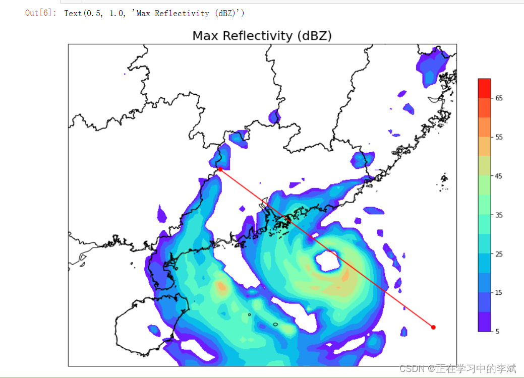

4. 插值dBZ至垂直剖面

# 插值前转化成对数
z_log = 10**(dbz/10.) # Use linear Z for interpolation
# 插值至垂直剖面
z_cross = vertcross(z_log, ht, wrfin=wrf_file,start_point=cross_start,end_point=cross_end,latlon=True, meta=True)
# 插值后转换回来
dbz_cross = 10.0 * np.log10(z_cross)# 前面的操作使变量丢失属性，将属性添加回去
dbz_cross.attrs.update(dbz.attrs)
dbz_cross.attrs["description"] = "radar reflectivity cross section"
dbz_cross.attrs["units"] = "dBZ"

5. 插值地形高度至cross line

# 插值地形高度至cross line
ter_line = interpline(ter, wrfin=wrf_file, start_point=cross_start,end_point=cross_end)

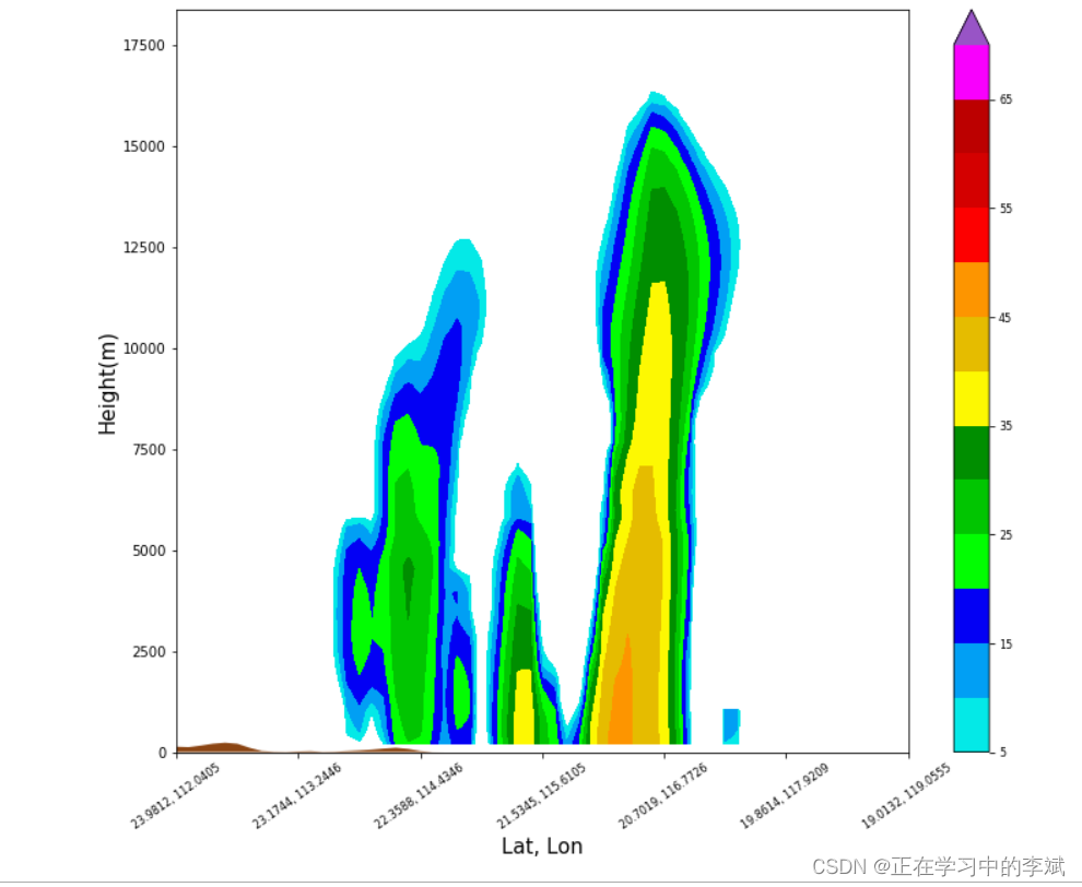
6.绘制垂直剖面dbz

# 插值地形高度至cross line
fig = plt.figure(figsize=(12,10))
ax_cross = fig.add_subplot(1,1,1)########################### 绘制垂直剖面dbz
dbz_levels = np.arange(5., 75., 5.)  # 14个区间# Create the color table found on NWS pages. # 14个区间
dbz_rgb = np.array([[4,233,231],[1,159,244], [3,0,244],[2,253,2], [1,197,1],[0,142,0], [253,248,2],[229,188,0], [253,149,0],[253,0,0], [212,0,0],[188,0,0],[248,0,253],[152,84,198]], np.float32) / 255.0#是一个辅助函数，可以帮助创建cmap和norm实例，其行为类似于Contourf的level和colors参数的行为
dbz_cmap, dbz_norm = from_levels_and_colors(dbz_levels, dbz_rgb,extend="max")xs = np.arange(0, dbz_cross.shape[-1], 1)
ys = to_np(dbz_cross.coords["vertical"])
dbz_np = to_np(dbz_cross) 
dbz_contours = ax_cross.contourf(xs,ys[0:90],dbz_np[0:90,:],levels=dbz_levels,cmap=dbz_cmap,norm=dbz_norm,extend="max")
# Add the color bar
cb_dbz = fig.colorbar(dbz_contours, ax=ax_cross)
cb_dbz.ax.tick_params(labelsize=8)# Fill in the mountain area
ht_fill = ax_cross.fill_between(xs, 0, to_np(ter_line),facecolor="saddlebrown")# Set the x-ticks to use latitude and longitude labels
coord_pairs = to_np(dbz_cross.coords["xy_loc"])
x_ticks = np.arange(coord_pairs.shape[0])
x_labels = [pair.latlon_str() for pair in to_np(coord_pairs)]thin = 10
ax_cross.set_xticks(x_ticks[::thin])
ax_cross.set_xticklabels(x_labels[::thin], rotation=35, fontsize=8)# Set the x-axis and  y-axis labels
ax_cross.set_xlabel("Lat, Lon", fontsize=15)
ax_cross.set_ylabel("Height(m)", fontsize=15)plt.savefig("wrf_cross_dbz.png")
plt.show()