Brian2 学习笔记(1)-Introduction to Brian part 1: Neurons

Now let’s go back to the good equations and actually run the simulation.

start_scope()tau = 10*ms
eqs = '''
dv/dt = (1-v)/tau : 1
'''G = NeuronGroup(1, eqs)
run(100*ms)

INFO       No numerical integration method specified for group 'neurongroup', using method 'exact' (took 0.04s). [brian2.stateupdaters.base.method_choice]

First off, ignore that start_scope() at the top of the cell. You’ll see that in each cell in this tutorial where we run a simulation. All it does is make sure that any Brian objects created before the function is called aren’t included in the next run of the simulation.

Secondly, you’ll see that there is an “INFO” message about not specifying the numerical integration method. This is harmless and just to let you know what method we chose, but we’ll fix it in the next cell by specifying the method explicitly.

So, what has happened here? Well, the command run(100*ms) runs the simulation for 100 ms. We can see that this has worked by printing the value of the variable v before and after the simulation.

start_scope()G = NeuronGroup(1, eqs, method='exact')
print('Before v = %s' % G.v[0])
run(100*ms)
print('After v = %s' % G.v[0])

Before v = 0.0
After v = 0.99995460007

By default, all variables start with the value 0. Since the differential equation is dv/dt=(1-v)/tauwe would expect after a while that v would tend towards the value 1, which is just what we see. Specifically, we’d expect v to have the value 1-exp(-t/tau). Let’s see if that’s right.

print('Expected value of v = %s' % (1-exp(-100*ms/tau)))

Expected value of v = 0.99995460007

Good news, the simulation gives the value we’d expect!

Now let’s take a look at a graph of how the variable v evolves over time.

start_scope()G = NeuronGroup(1, eqs, method='exact')
M = StateMonitor(G, 'v', record=True)run(30*ms)plot(M.t/ms, M.v[0])
xlabel('Time (ms)')
ylabel('v');

plt.show()

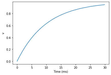
This time we only ran the simulation for 30 ms so that we can see the behaviour better. It looks like it’s behaving as expected, but let’s just check that analytically by plotting the expected behaviour on top.

start_scope()G = NeuronGroup(1, eqs, method='exact')
M = StateMonitor(G, 'v', record=0)run(30*ms)plot(M.t/ms, M.v[0], 'C0', label='Brian')
plot(M.t/ms, 1-exp(-M.t/tau), 'C1--',label='Analytic')
xlabel('Time (ms)')
ylabel('v')
legend();

plt.show()

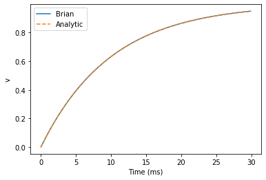
As you can see, the blue (Brian) and dashed orange (analytic solution) lines coincide.

In this example, we used the object StateMonitor object. This is used to record the values of a neuron variable while the simulation runs. The first two arguments are the group to record from, and the variable you want to record from. We also specify record=0. This means that we record all values for neuron 0. We have to specify which neurons we want to record because in large simulations with many neurons it usually uses up too much RAM to record the values of all neurons.

Now try modifying the equations and parameters and see what happens in the cell below.

start_scope()tau = 10*ms
eqs = '''
dv/dt = (sin(2*pi*100*Hz*t)-v)/tau : 1
'''# Change to Euler method because exact integrator doesn't work here
G = NeuronGroup(1, eqs, method='euler')
M = StateMonitor(G, 'v', record=0)G.v = 5 # initial valuerun(60*ms)plot(M.t/ms, M.v[0])
xlabel('Time (ms)')
ylabel('v');

plt.show()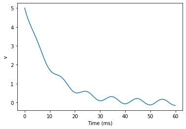

Adding spikes

So far we haven’t done anything neuronal, just played around with differential equations. Now let’s start adding spiking behaviour.

start_scope()tau = 10*ms
eqs = '''
dv/dt = (1-v)/tau : 1
'''G = NeuronGroup(1, eqs, threshold='v>0.8', reset='v = 0', method='exact')M = StateMonitor(G, 'v', record=0)
run(50*ms)
plot(M.t/ms, M.v[0])
xlabel('Time (ms)')
ylabel('v');

plt.show()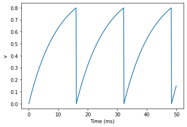

We’ve added two new keywords to the NeuronGroup declaration: threshold='v>0.8' and reset='v = 0'. What this means is that when v>0.8 we fire a spike, and immediately reset v = 0 after the spike. We can put any expression and series of statements as these strings.

As you can see, at the beginning the behaviour is the same as before until v crosses the threshold v>0.8 at which point you see it reset to 0. You can’t see it in this figure, but internally Brian has registered this event as a spike. Let’s have a look at that.

start_scope()G = NeuronGroup(1, eqs, threshold='v>0.8', reset='v = 0', method='exact')spikemon = SpikeMonitor(G)run(50*ms)print('Spike times: %s' % spikemon.t[:])

Spike times: [ 16.   32.1  48.2] ms

The SpikeMonitor object takes the group whose spikes you want to record as its argument and stores the spike times in the variable t. Let’s plot those spikes on top of the other figure to see that it’s getting it right.

start_scope()G = NeuronGroup(1, eqs, threshold='v>0.8', reset='v = 0', method='exact')statemon = StateMonitor(G, 'v', record=0)
spikemon = SpikeMonitor(G)run(50*ms)plot(statemon.t/ms, statemon.v[0])
for t in spikemon.t:axvline(t/ms, ls='--', c='C1', lw=3)
xlabel('Time (ms)')
ylabel('v');

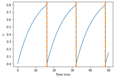
Here we’ve used the axvline command from matplotlib to draw an orange, dashed vertical line at the time of each spike recorded by the SpikeMonitor.

Now try changing the strings for threshold and reset in the cell above to see what happens.

Refractoriness

A common feature of neuron models is refractoriness. This means that after the neuron fires a spike it becomes refractory for a certain duration and cannot fire another spike until this period is over. Here’s how we do that in Brian.

start_scope()tau = 10*ms
eqs = '''
dv/dt = (1-v)/tau : 1 (unless refractory)
'''G = NeuronGroup(1, eqs, threshold='v>0.8', reset='v = 0', refractory=5*ms, method='exact')statemon = StateMonitor(G, 'v', record=0)
spikemon = SpikeMonitor(G)run(50*ms)plot(statemon.t/ms, statemon.v[0])
for t in spikemon.t:axvline(t/ms, ls='--', c='C1', lw=3)
xlabel('Time (ms)')
ylabel('v');

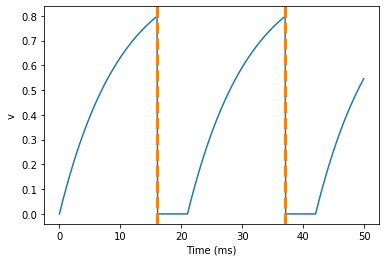
As you can see in this figure, after the first spike, v stays at 0 for around 5 ms before it resumes its normal behaviour. To do this, we’ve done two things. Firstly, we’ve added the keywordrefractory=5*ms to the NeuronGroup declaration. On its own, this only means that the neuron cannot spike in this period (see below), but doesn’t change how v behaves. In order to make vstay constant during the refractory period, we have to add (unless refractory) to the end of the definition of v in the differential equations. What this means is that the differential equation determines the behaviour of v unless it’s refractory in which case it is switched off.

Here’s what would happen if we didn’t include (unless refractory). Note that we’ve also decreased the value of tau and increased the length of the refractory period to make the behaviour clearer.

start_scope()tau = 5*ms
eqs = '''
dv/dt = (1-v)/tau : 1
'''G = NeuronGroup(1, eqs, threshold='v>0.8', reset='v = 0', refractory=15*ms, method='exact')statemon = StateMonitor(G, 'v', record=0)
spikemon = SpikeMonitor(G)run(50*ms)plot(statemon.t/ms, statemon.v[0])
for t in spikemon.t:axvline(t/ms, ls='--', c='C1', lw=3)
axhline(0.8, ls=':', c='C2', lw=3)
xlabel('Time (ms)')
ylabel('v')
print("Spike times: %s" % spikemon.t[:])

Spike times: [  8.   23.1  38.2] ms

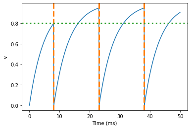
So what’s going on here? The behaviour for the first spike is the same: v rises to 0.8 and then the neuron fires a spike at time 8 ms before immediately resetting to 0. Since the refractory period is now 15 ms this means that the neuron won’t be able to spike again until time 8 + 15 = 23 ms. Immediately after the first spike, the value of v now instantly starts to rise because we didn’t specify (unless refractory) in the definition of dv/dt. However, once it reaches the value 0.8 (the dashed green line) at time roughly 8 ms it doesn’t fire a spike even though the threshold is v>0.8. This is because the neuron is still refractory until time 23 ms, at which point it fires a spike.

Note that you can do more complicated and interesting things with refractoriness. See the full documentation for more details about how it works.

Multiple neurons

So far we’ve only been working with a single neuron. Let’s do something interesting with multiple neurons.

start_scope()N = 100
tau = 10*ms
eqs = '''
dv/dt = (2-v)/tau : 1
'''G = NeuronGroup(N, eqs, threshold='v>1', reset='v=0', method='exact')
G.v = 'rand()'spikemon = SpikeMonitor(G)run(50*ms)plot(spikemon.t/ms, spikemon.i, '.k')
xlabel('Time (ms)')
ylabel('Neuron index');

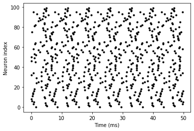
This shows a few changes. Firstly, we’ve got a new variable N determining the number of neurons. Secondly, we added the statement G.v = 'rand()' before the run. What this does is initialise each neuron with a different uniform random value between 0 and 1. We’ve done this just so each neuron will do something a bit different. The other big change is how we plot the data in the end.

As well as the variable spikemon.t with the times of all the spikes, we’ve also used the variable spikemon.i which gives the corresponding neuron index for each spike, and plotted a single black dot with time on the x-axis and neuron index on the y-value. This is the standard “raster plot” used in neuroscience.

Parameters

To make these multiple neurons do something more interesting, let’s introduce per-neuron parameters that don’t have a differential equation attached to them.

start_scope()N = 100
tau = 10*ms
v0_max = 3.
duration = 1000*mseqs = '''
dv/dt = (v0-v)/tau : 1 (unless refractory)
v0 : 1
'''G = NeuronGroup(N, eqs, threshold='v>1', reset='v=0', refractory=5*ms, method='exact')
M = SpikeMonitor(G)G.v0 = 'i*v0_max/(N-1)'run(duration)figure(figsize=(12,4))
subplot(121)
plot(M.t/ms, M.i, '.k')
xlabel('Time (ms)')
ylabel('Neuron index')
subplot(122)
plot(G.v0, M.count/duration)
xlabel('v0')
ylabel('Firing rate (sp/s)');

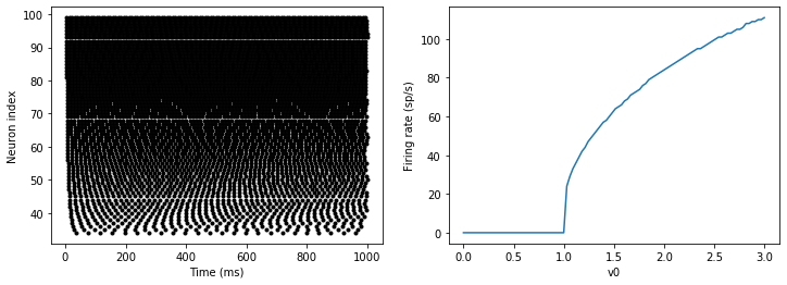
The line v0 : 1 declares a new per-neuron parameter v0 with units 1 (i.e. dimensionless).

The line G.v0 = 'i*v0_max/(N-1)' initialises the value of v0 for each neuron varying from 0 up to v0_max. The symbol i when it appears in strings like this refers to the neuron index.

So in this example, we’re driving the neuron towards the value v0 exponentially, but when vcrosses v>1, it fires a spike and resets. The effect is that the rate at which it fires spikes will be related to the value of v0. For v0<1 it will never fire a spike, and as v0 gets larger it will fire spikes at a higher rate. The right hand plot shows the firing rate as a function of the value of v0. This is the I-f curve of this neuron model.

Note that in the plot we’ve used the count variable of the SpikeMonitor: this is an array of the number of spikes each neuron in the group fired. Dividing this by the duration of the run gives the firing rate.

Stochastic neurons

Often when making models of neurons, we include a random element to model the effect of various forms of neural noise. In Brian, we can do this by using the symbol xi in differential equations. Strictly speaking, this symbol is a “stochastic differential” but you can sort of thinking of it as just a Gaussian random variable with mean 0 and standard deviation 1. We do have to take into account the way stochastic differentials scale with time, which is why we multiply it bytau**-0.5 in the equations below (see a textbook on stochastic differential equations for more details). Note that we also changed the method keyword argument to use 'euler' (which stands for the Euler-Maruyama method); the 'exact' method that we used earlier is not applicable to stochastic differential equations.

start_scope()N = 100
tau = 10*ms
v0_max = 3.
duration = 1000*ms
sigma = 0.2eqs = '''
dv/dt = (v0-v)/tau+sigma*xi*tau**-0.5 : 1 (unless refractory)
v0 : 1
'''G = NeuronGroup(N, eqs, threshold='v>1', reset='v=0', refractory=5*ms, method='euler')
M = SpikeMonitor(G)G.v0 = 'i*v0_max/(N-1)'run(duration)figure(figsize=(12,4))
subplot(121)
plot(M.t/ms, M.i, '.k')
xlabel('Time (ms)')
ylabel('Neuron index')
subplot(122)
plot(G.v0, M.count/duration)
xlabel('v0')
ylabel('Firing rate (sp/s)');

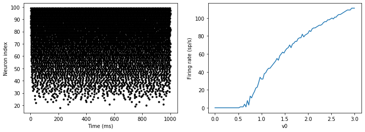
That’s the same figure as in the previous section but with some noise added. Note how the curve has changed shape: instead of a sharp jump from firing at rate 0 to firing at a positive rate, it now increases in a sigmoidal fashion. This is because no matter how small the driving force the randomness may cause it to fire a spike.

End of tutorial

That’s the end of this part of the tutorial. The cell below has another example. See if you can work out what it is doing and why. Try adding a StateMonitor to record the values of the variables for one of the neurons to help you understand it.

You could also try out the things you’ve learned in this cell.

Once you’re done with that you can move on to the next tutorial on Synapses.

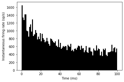
start_scope()N = 1000
tau = 10*ms
vr = -70*mV
vt0 = -50*mV
delta_vt0 = 5*mV
tau_t = 100*ms
sigma = 0.5*(vt0-vr)
v_drive = 2*(vt0-vr)
duration = 100*mseqs = '''
dv/dt = (v_drive+vr-v)/tau + sigma*xi*tau**-0.5 : volt
dvt/dt = (vt0-vt)/tau_t : volt
'''reset = '''
v = vr
vt += delta_vt0
'''G = NeuronGroup(N, eqs, threshold='v>vt', reset=reset, refractory=5*ms, method='euler')
spikemon = SpikeMonitor(G)G.v = 'rand()*(vt0-vr)+vr'
G.vt = vt0run(duration)_ = hist(spikemon.t/ms, 100, histtype='stepfilled', facecolor='k', weights=ones(len(spikemon))/(N*defaultclock.dt))
xlabel('Time (ms)')
ylabel('Instantaneous firing rate (sp/s)');