本文主要是介绍Retinaface训练超参数调优,希望对大家解决编程问题提供一定的参考价值,需要的开发者们随着小编来一起学习吧!
训练20遍数据集跑出的效果
from __future__ import print_functionimport argparse
import math
import osimport optuna
import torch
import torch.backends.cudnn as cudnn
import torch.optim as optim
import torch.utils.data as datafrom data import WiderFaceDetection, detection_collate, preproc, cfg_mnet, cfg_re50
from layers.functions.prior_box import PriorBox
from layers.modules import MultiBoxLoss
from models.retinaface import RetinaFace# 解析命令行参数
parser = argparse.ArgumentParser(description='Retinaface Training')
parser.add_argument('--training_dataset', default='./data/lst/train/label.txt', help='训练数据集目录')
parser.add_argument('--network', default='resnet50', help='Backbone 网络选择: mobile0.25 或 resnet50')
parser.add_argument('--num_workers', default=4, type=int, help='数据加载时的工作线程数')
parser.add_argument('--resume_net', default=None, help='重新训练时的已保存模型路径')
parser.add_argument('--resume_epoch', default=0, type=int, help='重新训练时的迭代轮数')
parser.add_argument('--save_folder', default='./weights/', help='保存检查点模型的目录')# 解析参数
args = parser.parse_args()# 如果 save_folder 目录不存在,则创建它
if not os.path.exists(args.save_folder):os.mkdir(args.save_folder)# 根据选择的网络初始化配置
cfg = None
if args.network == "mobile0.25":cfg = cfg_mnet
elif args.network == "resnet50":cfg = cfg_re50# 设置 RGB 平均值、类别数、图像维度等
rgb_mean = (104, 117, 123)  # BGR 顺序
num_classes = 2
img_dim = cfg['image_size']
num_gpu = cfg['ngpu']
batch_size = cfg['batch_size']
max_epoch = cfg['epoch']
gpu_train = cfg['gpu_train']num_workers = args.num_workers
training_dataset = args.training_dataset
save_folder = args.save_folder# 超参数优化目标函数
def objective(trial):# 超参数搜索空间initial_lr = trial.suggest_float('lr', 1e-5, 1e-2, log=True)momentum = trial.suggest_float('momentum', 0.7, 0.99)weight_decay = trial.suggest_float('weight_decay', 1e-5, 1e-2, log=True)gamma = trial.suggest_float('gamma', 0.1, 0.5, log=True)# 初始化 RetinaFace 模型net = RetinaFace(cfg=cfg)# 如果指定了 resume_net,加载预训练权重if args.resume_net is not None:state_dict = torch.load(args.resume_net)from collections import OrderedDictnew_state_dict = OrderedDict()for k, v in state_dict.items():head = k[:7]if head == 'module.':name = k[7:]  # 移除 `module.`else:name = knew_state_dict[name] = vnet.load_state_dict(new_state_dict)# 如果有多个 GPU 可用,使用 DataParallel 进行并行训练if num_gpu > 1 and gpu_train:net = torch.nn.DataParallel(net).cuda()else:net = net.cuda()cudnn.benchmark = True# 定义优化器、损失函数和先验框optimizer = optim.SGD(net.parameters(), lr=initial_lr, momentum=momentum, weight_decay=weight_decay)criterion = MultiBoxLoss(num_classes, 0.35, True, 0, True, 7, 0.35, False)priorbox = PriorBox(cfg, image_size=(img_dim, img_dim))with torch.no_grad():priors = priorbox.forward()priors = priors.cuda()# 训练函数def train():net.train()epoch = 0 + args.resume_epochdataset = WiderFaceDetection(training_dataset, preproc(img_dim, rgb_mean))epoch_size = math.ceil(len(dataset) / batch_size)max_iter = max_epoch * epoch_sizestepvalues = (cfg['decay1'] * epoch_size, cfg['decay2'] * epoch_size)step_index = 0start_iter = args.resume_epoch * epoch_size if args.resume_epoch > 0 else 0for iteration in range(start_iter, max_iter):if iteration % epoch_size == 0:batch_iterator = iter(data.DataLoader(dataset, batch_size, shuffle=True, num_workers=num_workers,collate_fn=detection_collate))epoch += 1if iteration in stepvalues:step_index += 1lr = adjust_learning_rate(optimizer, gamma, epoch, step_index, iteration, epoch_size)images, targets = next(batch_iterator)images = images.cuda()targets = [anno.cuda() for anno in targets]out = net(images)optimizer.zero_grad()loss_l, loss_c, loss_landm = criterion(out, priors, targets)loss = cfg['loc_weight'] * loss_l + loss_c + loss_landmloss.backward()optimizer.step()return loss.item()# 学习率调整函数def adjust_learning_rate(optimizer, gamma, epoch, step_index, iteration, epoch_size):warmup_epoch = 5if epoch < warmup_epoch:lr = initial_lr * (iteration + 1) / (epoch_size * warmup_epoch)else:lr = initial_lr * 0.5 * (1 + math.cos(math.pi * (epoch - warmup_epoch) / (max_epoch - warmup_epoch)))for param_group in optimizer.param_groups:param_group['lr'] = lrreturn lr# 训练并返回损失final_loss = train()# 将超参数和对应的损失写入文件with open('best.txt', 'a') as f:f.write(f"Trial {trial.number} - Loss: {final_loss}\n")f.write(f"lr: {initial_lr}, momentum: {momentum}, weight_decay: {weight_decay}, gamma: {gamma}\n\n")return final_lossif __name__ == '__main__':# 使用 Optuna 进行超参数优化study = optuna.create_study(direction='minimize')study.optimize(objective, n_trials=20)print('最佳超参数:')print(study.best_params)# 将最佳超参数写入文件with open('best.txt', 'a') as f:f.write('最佳超参数:\n')f.write(str(study.best_params))f.write('\n')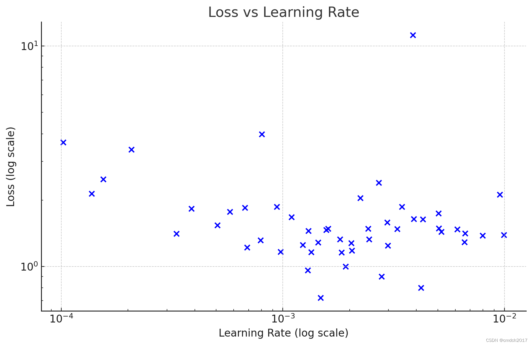
Trial	Loss	Learning Rate (lr)
0	1.474661	0.006130
1	2.118352	0.009536
2	0.720860	0.001478
3	1.219791	0.000690
4	2.139611	0.000137
5	2.485054	0.000155
6	3.654128	0.000102
7	1.276526	0.002037
8	3.393638	0.000207
9	1.449489	0.001304
10	1.539526	0.000506
11	1.774117	0.000576
12	2.403089	0.002708
13	1.850937	0.000673
14	1.411137	0.000331
15	0.963467	0.001294
16	1.245503	0.002975
17	1.674727	0.001095
18	1.468113	0.001567
19	0.801777	0.004197
20	11.193202	0.003866
21	1.638056	0.004286
22	1.181070	0.002046
23	1.436263	0.005183
24	1.868375	0.000939
25	1.384036	0.007968
26	1.327896	0.001810
27	0.900618	0.002786
28	1.587448	0.002961
29	1.414236	0.006639
30	1.640772	0.003894
31	1.167393	0.000975
32	1.327571	0.002453
33	1.163059	0.001341
34	1.491638	0.005048
35	1.831493	0.000386
36	3.975567	0.000802
37	1.390656	0.009954
38	1.485421	0.001599
39	2.045896	0.002233
40	1.480700	0.003282
41	1.251927	0.001231
42	1.286666	0.001444
43	1.157723	0.001841
44	1.000185	0.001921
45	1.868337	0.003445
46	1.291534	0.006600
47	1.486465	0.002422
48	1.743561	0.005034
49	1.316136	0.000792
import pandas as pd
import matplotlib.pyplot as plt# Creating a DataFrame with the extracted data
data = {"Trial": list(range(50)),"Loss": [1.474661, 2.118352, 0.720860, 1.219791, 2.139611, 2.485054, 3.654128, 1.276526, 3.393638, 1.449489, 1.539526, 1.774117, 2.403089, 1.850937, 1.411137, 0.963467, 1.245503, 1.674727, 1.468113, 0.801777, 11.193202, 1.638056, 1.181070, 1.436263, 1.868375, 1.384036, 1.327896, 0.900618, 1.587448, 1.414236, 1.640772, 1.167393, 1.327571, 1.163059, 1.491638, 1.831493, 3.975567, 1.390656, 1.485421, 2.045896, 1.480700, 1.251927, 1.286666, 1.157723, 1.000185, 1.868337, 1.291534, 1.486465, 1.743561, 1.316136],"Learning Rate (lr)": [0.006130, 0.009536, 0.001478, 0.000690, 0.000137, 0.000155, 0.000102, 0.002037, 0.000207, 0.001304,0.000506, 0.000576, 0.002708, 0.000673, 0.000331, 0.001294, 0.002975, 0.001095, 0.001567, 0.004197,0.003866, 0.004286, 0.002046, 0.005183, 0.000939, 0.007968, 0.001810, 0.002786, 0.002961, 0.006639,0.003894, 0.000975, 0.002453, 0.001341, 0.005048, 0.000386, 0.000802, 0.009954, 0.001599, 0.002233,0.003282, 0.001231, 0.001444, 0.001841, 0.001921, 0.003445, 0.006600, 0.002422, 0.005034, 0.000792]
}df = pd.DataFrame(data)# Sorting the dataframe by learning rate for a smooth line plot
df_sorted = df.sort_values(by="Learning Rate (lr)")# Extracting sorted data
sorted_learning_rates = df_sorted["Learning Rate (lr)"]
sorted_losses = df_sorted["Loss"]# Plotting line chart
plt.figure(figsize=(10, 6))
plt.plot(sorted_learning_rates, sorted_losses, marker='o', linestyle='-', color='blue')
plt.xscale('log')  # Using logarithmic scale for learning rate to better visualize the range
plt.yscale('log')  # Using logarithmic scale for loss to better visualize the range
plt.title('Loss vs Learning Rate')
plt.xlabel('Learning Rate (log scale)')
plt.ylabel('Loss (log scale)')
plt.grid(True)
plt.show()
要确定进一步训练的最佳学习率范围,我们可以通过以下几点分析学习率与损失之间的关系:
低损失区域:找出在较低损失值对应的学习率范围。
稳定性:选择一个损失值较低且稳定的学习率范围。
从已提供的数据中,我们可以观察哪些学习率对应较低的损失值:
最低损失值为0.720860,出现在学习率为0.001478。
其他较低损失值(低于1.0)出现在以下学习率:
0.004197 对应损失 0.801777
0.002786 对应损失 0.900618
0.001294 对应损失 0.963467
综合考虑损失较低和稳定性,学习率范围可以集中在0.001到0.005之间。具体建议如下:
初步范围:0.001到0.005
更精细的范围:由于在0.001478、0.004197和0.002786处有较低的损失,可以进一步缩小到0.001到0.002和0.004到0.005之间。
进一步训练建议
在0.001到0.002之间试验更多的学习率值,例如0.0011, 0.0015, 0.0018等。
在0.004到0.005之间试验,例如0.0042, 0.0045, 0.0048等。
通过这些步骤,您可以更准确地找到最佳学习率,从而进一步降低损失,提高模型的性能
这篇关于Retinaface训练超参数调优的文章就介绍到这儿,希望我们推荐的文章对编程师们有所帮助!


