talib 买卖信号_如何产生股票交易的买卖信号

回归和分类生成买/卖信号(Regression & Classification to generate buy/sell signals)

Moving average rule says that, buy and sell signals are generated by two moving averages of the level of the index-a long-period average and a short-period average. This strategy is expressed as buying (or selling) in its simplest form; which means when the short-period moving average rises above (or falls below) the long-period moving average. The idea behind computing moving averages it to smooth out an otherwise volatile series. When the short-period moving average penetrates the long-period moving average, a trend is considered to be initiated.

中号oving平均规则认为，买卖信号是由指数长周期平均和短周期平均水平的两条移动均线产生。 这种策略以最简单的形式表示为购买(或出售)。 这意味着当短期移动平均线高于(或低于)长期移动平均线时。 计算移动平均线背后的想法是将其平滑以消除本来不稳定的序列。 当短期移动平均线穿入长期移动平均线时，就认为趋势已经开始。

Here, with a simple example, we have shown as how to generate report on buy/sell signals and visualize the chart.

在这里，通过一个简单的示例，我们展示了如何生成有关买/卖信号的报告并可视化图表。

print("....Data Loading...."); print();
print('\033[4mCrude Oil Spot Price\033[0m');
data = web.DataReader('CL=F', data_source = 'yahoo', start = '2000-01-01');
data;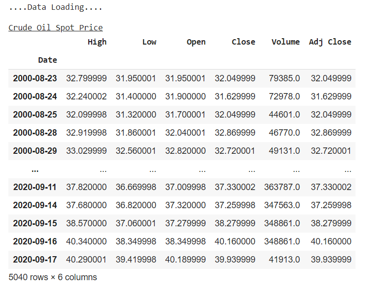

Let’s focus on closing price of daily stock.

让我们专注于每日股票的收盘价。

df = data[['Close']];
# Plot the closing price
df.Close.plot(figsize=(10, 5));
plt.ylabel("Prices (USD)"); plt.title("Crude Oil Price Series");
plt.show();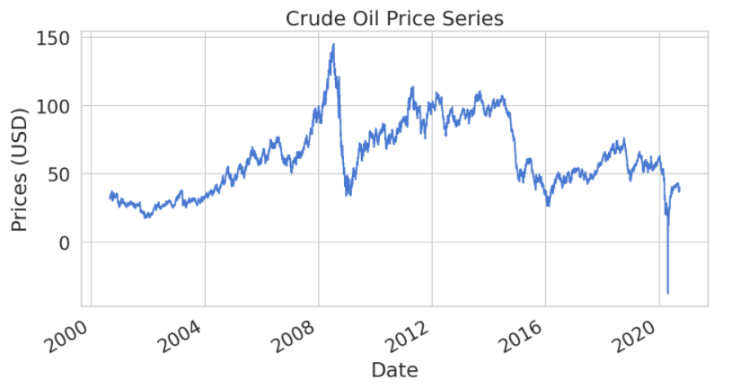

解释变量 (Explanatory variables)

To find the price movement of a stock, we will use two EMAs of different time period. We have taken exponential moving average (ema); in simple moving average (sma), each value in the time period carries equal weight, and values outside of the time period are not included in the average. However, the ema is a cumulative calculation, including all data. Past values have a diminishing contribution to the average, while more recent values have a greater contribution. This method allows the moving average to be more responsive to changes in the data.

为了找到股票的价格走势，我们将使用两个不同时间段的EMA。 我们采用了指数移动平均线(ema)； 在简单移动平均值(sma)中，时间段中的每个值都具有相等的权重，并且该时间段之外的值不包括在平均值中。 但是，ema是包括所有数据的累积计算。 过去的值对平均值的贡献减小，而最近的值对平均值的贡献更大。 这种方法使移动平均值对数据的变化更加敏感。

df['ema10'] = (df['Close'].ewm(span=10,adjust=True,ignore_na=True).mean());
df['ema20'] = (df['Close'].ewm(span=20,adjust=True,ignore_na=True).mean());
df['price_tomorrow'] = df['Close'].shift(-1);
df.dropna(inplace=True);
X = df[['ema10', 'ema20']]; y = df['price_tomorrow'];

用原始数据绘制EMA (Plot EMA with original data)

fig = go.Figure(data=[go.Candlestick(x=data.index[-100:],
open=data['Open'][-100:], high=data['High'][-100:], low=data['Low'][-100:], close=data['Close'][-100:])]);
fig.add_trace(go.Scatter(x = df.index[-100:], y = df.ema10[-100:], marker = dict(color = "blue"), name = "EMA10"));
fig.add_trace(go.Scatter(x = df.index[-100:], y = df.ema20[-100:], marker = dict(color = "gray"), name = "EMA10"));
fig.update_xaxes(showline=True, linewidth=2, linecolor='black', mirror=True);
fig.update_yaxes(showline=True, linewidth=2, linecolor='black', mirror=True);
fig.update_layout(autosize = False, width = 1200, height = 600);
fig.update_layout(title='Crude oil prices, yaxis_title='(US$)');
fig.show();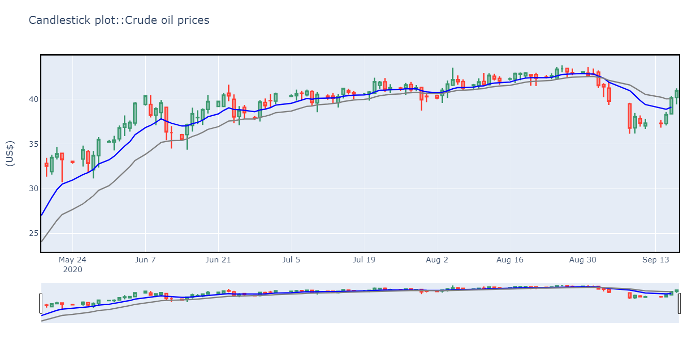

Here, shorter the period, the more weight is given to recent prices. In fact a short time period generates a line closely following the actual candles on the chart. Visually this means that there are more occurrences of the price moving above or below the EMA which can be interpreted as a signal to open or close a position.

在这里，时间越短，对近期价格的重视就越大。 实际上，很短的一段时间会在图表上的实际蜡烛线附近紧贴一条线。 从视觉上看，这意味着有更多的价格在EMA上方或下方移动，这可以解释为开仓或平仓的信号。

时间序列数据分割 (Time series data split)

# Split the data into train and test data set
tscv = TimeSeriesSplit();
print(tscv);
TimeSeriesSplit(max_train_size = 0.80, n_splits=5);
for train_index, test_index in tscv.split(X):
   #print("TRAIN:", train_index, "TEST:", test_index);
   X_train, X_test = X[train_index], X[test_index];
   y_train, y_test = y[train_index], y[test_index];print('Length train set: {}'.format(len(y_train)));
print('Length test set: {}'.format(len(y_test)));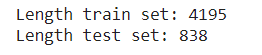

回归规则 (Regression rule)

# Create a linear regression model
model = ElasticNet(max_iter=5000, random_state=0).fit(X_train, y_train);
print("Linear Regression model:");
print("Crude oil Price (y) = %.2f * 10 Days Moving Average (x1) \
+ %.2f * 20 Days Moving Average (x2) \
+ %.2f (constant)" % (model.coef_[0], model.coef_[1], model.intercept_));

绘制实际和预测输出 (Plot actual and predicted output)

y_pred = DataFrame(model.predict(X_test), index = df[-len(y_test):].index, columns = ['price']);
y_test = DataFrame(y_test, index = df[-len(y_test):].index, columns = ['price']);fig = go.Figure();
fig.add_trace(go.Scatter(x = y_pred.index, y = y_pred.price,
marker = dict(color ="red"), name = "Actual price"));
fig.add_trace(go.Scatter(x = y_test.index, y = y_test.price, marker=dict(color = "green"), name = "Predicted price"));
fig.update_xaxes(showline = True, linewidth = 2, linecolor='black', mirror = True, showspikes = True,);
fig.update_yaxes(showline = True, linewidth = 2, linecolor='black', mirror = True, showspikes = True,);
fig.update_layout(title= "Crude oil price (predicted vs actual", yaxis_title = 'price (US$)', hovermode = "x", hoverdistance = 100, spikedistance = 1000);
fig.update_layout(autosize = False, width = 1000, height = 400,);
fig.show();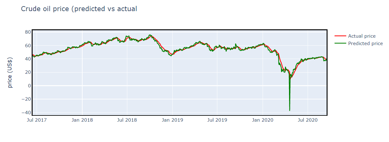

测试精度 (Test accuracy)

accuracy = model.score(X_test, y_test);
print("Accuracy: ", round(accuracy*100,2).astype(str) + '%');

oil = DataFrame();
oil['price'] = df[-len(y_test):]['Close'];
oil['pred_next_day'] = y_pred;
oil['actual_price_next_day'] = y_test;
oil['returns'] = oil['price'].pct_change().shift(-1);
oil['signal'] = np.where(oil.pred_next_day.shift(1) < oil.pred_next_day,1,0);
oil['strategy_returns'] = oil.signal * oil['returns'];((oil['strategy_returns']+1).cumprod()).plot(figsize=(10,5));
plt.ylabel('Cumulative Returns');
plt.show();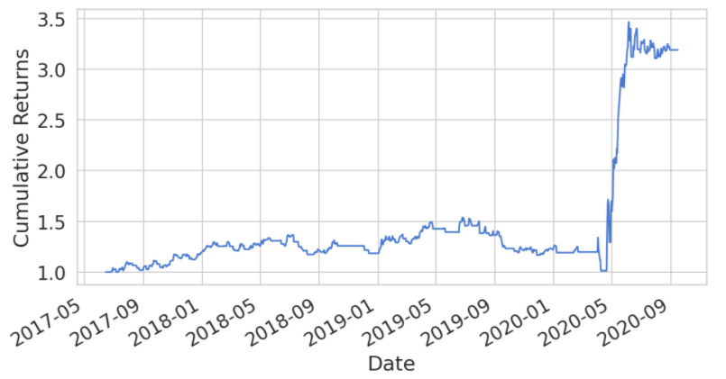

The Sharpe ratio is a well-known and well-reputed measure of risk-adjusted return on an investment or portfolio, developed by the economist William Sharpe.

夏普(Sharpe)比率是经济学家威廉·夏普(William Sharpe)提出的一种众所周知的，声誉良好的衡量风险的投资或投资组合调整收益的方法。

The Formula for the Sharpe Ratio is:

夏普比率的公式是：

Average return / Std dev of return

平均回报率/标准回报率

• Usually, any Sharpe ratio > 1.0 is considered acceptable.
  通常，任何大于1.0的Sharpe比率都可以接受。
• A ratio > 2.0 is rated as very good.
  比率> 2.0被评为非常好。
• A ratio of 3.0 or higher is considered excellent.
  3.0或更高的比率被认为是极好的。
• A ratio < 1.0 is considered sub-optimal.
  比率<1.0被认为是次优的。

买卖报告 (Buy/Sell Report)

df.loc[:,'pred_price'] = model.predict(df[['ema10', 'ema20']]);
df.loc[:,'signal'] = np.where(df.pred_price.shift(1) < df.pred_price,"Buy","Sell");
df.loc[:,'price_direction'] = df['signal'].replace(('Sell', 'Buy'), (0, 1));
df.tail();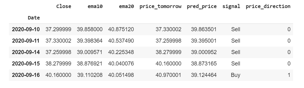

买/卖信号图 (Buy/Sell signals plot)

buys = df.loc[df['price_direction'] == 1]; sells = df.loc[df['price_direction'] == 0];# Plot
fig = plt.figure(figsize=(20, 5));
plt.plot(df.index, df['Close'], lw=2., label='Price');# Plot the buy and sell signals on the same plot
plt.plot(buys.index, df.loc[buys.index]['Close'], '^', markersize=5, color='k', lw=2., label='Buy');
plt.plot(sells.index, df.loc[sells.index]['Close'], 'v', markersize = 5, color='g', lw=2., label='Sell');
plt.ylabel('Price (USD)'); plt.xlabel('Date');
plt.title('Buy and Sell signals plot'); plt.legend(loc='best');# Display everything
plt.show()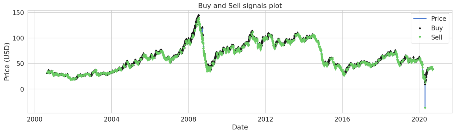

分类规则 (Classification rule)

# creating predictors and target variables for classification
print('Data shape:', df.shape); print();
X = np.array(df[['ema10', 'ema20']]);# Target variable
y = np.array(df['price_direction']);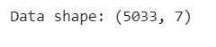

时间序列分割 (Time series split)

tscv = TimeSeriesSplit()
#print(tscv)
TimeSeriesSplit(max_train_size = 0.80, n_splits=5)
for train_index, test_index in tscv.split(X):
    #print("TRAIN:", train_index, "TEST:", test_index)
    X_train, X_test = X[train_index], X[test_index]
    y_train, y_test = y[train_index], y[test_index]print('Length train set: {}'.format(len(y_train)))
print('Length test set: {}'.format(len(y_test)))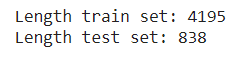

逻辑回归 (Logistic Regression)

print('\033[4mLogistic Regression\033[0m')
clf = LogisticRegression(solver='liblinear', C=0.05, random_state=0
).fit (X_train,y_train);
model_scores = cross_val_score(clf, X_train, y_train, cv=5);
model_mean = model_scores.mean();
print ('Accuracy score (%):', model_mean*100);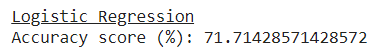

预测与准确性 (Prediction & accuracy)

y_pred = clf.predict(X_test)
# evaluate predictions
accuracy = accuracy_score(y_test, y_pred)
print("Accuracy: %.2f%%" % (accuracy * 100.0))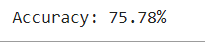

分类报告 (Classification report)

print('Confusion matrix:'); print(confusion_matrix(y_test, y_pred)); print(); print ('Classification report:'); print (classification_report(y_test, y_pred));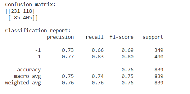

The recall means how many of this class we find over the whole number of element of this class. The precision here is how many are correctly classified among that class. The f1-score is the harmonic mean between precision & recall. The support is the number of occurrence of the given class in our data.

召回意味着我们可以在该类的全部元素中找到多少个此类。 这里的精度是在该类中正确分类的数量。 f1分数是精度和查全率之间的谐波平均值。 支持是给定类在我们的数据中出现的次数。

结论 (Conclusion)

We have shown here a simplified version of generating buy/sell signals based on moving average. This is a simple and fundamental process. Other technical indicators such as MACD, ROC etc. can be added based on trading strategy.

我们在这里显示了根据移动平均值生成买/卖信号的简化版本。 这是一个简单而基本的过程。 可以根据交易策略添加其他技术指标，例如MACD，ROC等。

Connect me here.

在这里连接我。

Note: The programs described here are experimental and should be used with caution for any commercial purpose. All such use at your own risk.

注意：此处描述的程序是实验性的，出于商业目的应谨慎使用。 所有此类使用后果自负。